Page 151 - Autonomous Mobile Robots

134 Autonomous Mobile Robots

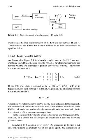
Du, Dv INS Position
IMU equations velocity
Position
velocity
Nav
GPS filter
Position, velocity

FIGURE 3.4 Block diagram of a loosely coupled GPS aided INS.

must be specified for implementation of the EKF are the matrices H and R.
These matrices are distinct for the two methods to be discussed and will be
specified below.

3.5.2.1 Loosely coupled system
As illustrated in Figure 3.4, in a loosely coupled system, the EKF measure-
ments are the GPS position (or velocity or both). Residual measurements are
formed with the INS estimates of position (or velocity or both). The position
measurement residual is

   
1 0 0 δn
y = p gps − p ins =  0 1 0   δe  + η x (3.69)
0 0 1 δd

T T T T T T
If the INS error state is ordered as δx =[δp , δv , δρ , x , x ] as in
g
a
Equation (3.68); then, for Step 4 of the EKF algorithm, the linearized position
measurement matrix is
H k =[I, 0]

whereI isa3×3identitymatrixand0isa3×12matrixofzeros. Inthisapproach,
the receiver clock model and associated error states need not be included in the
EKF model, as the receiver has already accounted for the receiver clock bias in
the estimation of the receiver antenna position.
For the implemented system to attain performance near that predicted the-
oretically, it is critical for the designer to understand at least the following
practical issues:
Correlated GPS position error vector: As discussed in Section 3.3.2
and demonstrated in Example 3.2, at any given epoch, the components of

© 2006 by Taylor & Francis Group, LLC

FRANKL: “dk6033_c003” — 2006/3/31 — 16:42 — page 134 — #36