Page 156 - Autonomous Mobile Robots

Data Fusion via Kalman Filter 139

Vel. error, m/sec 0
1

– 1
0 10 20 30 40
0.2
Bias errors 0

– 0.2
0 10 20 30 40
2
Yaw error, deg 0

– 2
0 10 20 30 40
Time, t (sec)

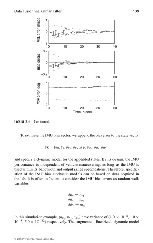
FIGURE 3.6 Continued.

To estimate the IMU bias vector, we append the bias error to the state vector

δx =[δn, δe, δv n , δv e , δψ, δa u , δa v , δω r ]

and specify a dynamic model for the appended states. By its design, the IMU
performance is independent of vehicle maneuvering, as long as the IMU is
used within its bandwidth and output range specifications. Therefore, specific-
ation of the IMU bias stochastic models can be based on data acquired in
the lab. It is often sufficient to consider the IMU bias errors as random walk
variables

δ˙a u = n b 1
δ˙a v = n b 2
δ ˙ω r = n b 3

) have variance of (1.0 × 10 −8
In this simulation example, (n b 1 , n b 2 , n b 3 , 1.0 ×
10 −8 , 5.0 × 10 −12 ) respectively. The augmented, linearized, dynamic model

© 2006 by Taylor & Francis Group, LLC

FRANKL: “dk6033_c003” — 2006/3/31 — 16:42 — page 139 — #41