Page 155 - Autonomous Mobile Robots

138 Autonomous Mobile Robots

15

10
y (m) 5

0
– 5
0 200 400 600 800
x (m)

5
Estimation error (m) 0

– 5
0 10 20 30 40
Time, t (sec)

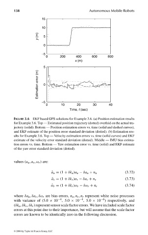
FIGURE 3.6 EKF based GPS solutions for Example 3.6. (a) Position estimation results
for Example 3.6. Top — Estimated position trajectory (dotted) overlaid on the actual tra-
jectory (solid). Bottom — Position estimation errors vs. time (solid and dashed curves),
and EKF estimate of the position error standard deviation (dotted). (b) Estimation res-
ults for Example 3.6. Top — Velocity estimation errors vs. time (solid curves) and EKF
estimate of the velocity error standard deviation (dotted). Middle — IMU bias estima-
tion errors vs. time. Bottom — Yaw estimation error vs. time (solid) and EKF estimate
of the yaw error standard deviation (dotted).

values (a u , a v , ω r ) are:

˜ a u = (1 + δk u )a u − δa u + n u (3.72)
˜ a v = (1 + δk v )a v − δa v + n v (3.73)
˜ ω r = (1 + δk r )ω r − δω r + n r (3.74)

where δa u , δa v , δω r are bias errors, n u , n v , n r represent white noise processes
with variance of (5.0 × 10 −4 , 5.0 × 10 −4 , 5.0 × 10 −6 ) respectively, and
(δk u , δk v , δk r ) represent sensor scale factor errors. We have included scale factor
errors at this point due to their importance, but will assume that the scale factor
errors are known to be identically zero in the following discussion.

© 2006 by Taylor & Francis Group, LLC

FRANKL: “dk6033_c003” — 2006/3/31 — 16:42 — page 138 — #40