Page 194 - Autonomous Mobile Robots

178 Autonomous Mobile Robots

1/RMS(/m)

250
200

150
100

50
8
7
6
0 5
– 4 4
– 3 – 2 – 1 3
0 1 2 1 2 y(m)
x(m) 3 4 0
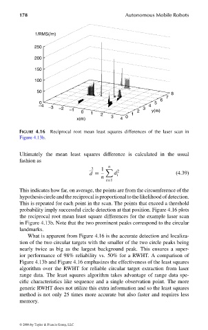
FIGURE 4.16 Reciprocal root mean least squares differences of the laser scan in
Figure 4.13b.

Ultimately the mean least squares difference is calculated in the usual
fashion as
n
_2 1 2
d = d i (4.39)
n
i=1
This indicates how far, on average, the points are from the circumference of the
hypothesiscircleandthereciprocalisproportionaltothelikelihoodofdetection.
This is repeated for each point in the scan. The points that exceed a threshold
probability imply successful circle detection at that position. Figure 4.16 plots
the reciprocal root mean least square differences for the example laser scan
in Figure 4.13b. Note that the two prominent peaks correspond to the circular
landmarks.
What is apparent from Figure 4.16 is the accurate detection and localiza-
tion of the two circular targets with the smaller of the two circle peaks being
nearly twice as big as the largest background peak. This ensures a super-
ior performance of 98% reliability vs. 50% for a RWHT. A comparison of
Figure 4.13b and Figure 4.16 emphasizes the effectiveness of the least squares
algorithm over the RWHT for reliable circular target extraction from laser
range data. The least squares algorithm takes advantage of range data spe-
cific characteristics like sequence and a single observation point. The more
generic RWHT does not utilize this extra information and so the least squares
method is not only 25 times more accurate but also faster and requires less
memory.

© 2006 by Taylor & Francis Group, LLC

FRANKL: “dk6033_c004” — 2006/3/31 — 16:42 — page 178 — #30