Page 231 - Autonomous Mobile Robots

216 Autonomous Mobile Robots

5.7 ROBUST STABILIZATION —PART II
In this section we consider the robust stabilization problem for nonholonomic
systems in the presence of measurement errors and exogenous disturbances.
This problem has been only partly investigated, and several attempts have been
made to study the robustness properties of existing control laws or to robustify
given controllers [34,53,57]. Most of the robust stabilization results and invest-
igations focus on the problems of parametric uncertainties or model errors, see
for example, [58] where the problem of local robust stabilization by means of
time-varying control laws have been studied; [57], where a similar problem
has been addressed using the class of discontinuous control laws discussed in
Section 5.4 and [8,24] where several types of hybrid control laws have been used
to achieve local robustness against unknown parameters or unmodelled dynam-
ics. On the other hand, the fundamental problems of robustness in the presence
of sensor noise, external disturbances, and actuator disturbances have been
l only partially addressed, see for example, [33,53]. These problems are of spe-
cial interest and relevance whenever discontinuous control laws are employed,
as for such control laws classical robustness results and Lyapunov theory are not
directly applicable, see however Reference 59, where a discontinuous control
law, possessing a Lyapunov stability property, has been constructed. In what
follows we make use of the class of discontinuous control laws presented in
Section 5.4 and we show how, adding a proper modification together with a
hybrid variable, it is possible to obtain a closed loop system with global sta-
bility properties and which is globally robust against measurement noises and
exogenous disturbances. The proposed controller takes inspiration from the
results in References 33, 60, and 61.

5.7.1 The Local Controller
2
n
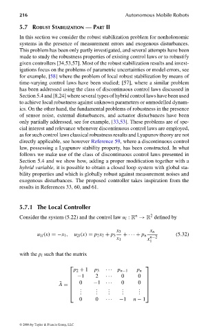
Consider the system (5.22) and the control law u l : R → R defined by
x 3 x n
u 1l (x) =−x 1 , u 2l (x) = p 2 x 2 + p 3 + ··· + p n n−2 (5.32)
x 1 x
1
with the p i such that the matrix

p 2 + 1 p 3 ··· p n−1 p n
 
−1 2 0 0
 ··· 
 
0 −1 0 0
¯  ··· 
. . . .
A =  
. . . . .
 . 
 . . . . . 
0 0 ··· −1 n − 1
© 2006 by Taylor & Francis Group, LLC

FRANKL: “dk6033_c005” — 2006/3/31 — 16:42 — page 216 — #30