Page 234 - Autonomous Mobile Robots

Stabilization of Nonholonomic Systems 219

the large has been advocated in several papers, and typically in the context
of stabilization of unstable equilibria of mechanical systems. However, what
makes the present result interesting is that we aim at achieving robust asymptotic
stability rather than asymptotic stability.

5.8 ROBUST STABILITAZION —PART III
In the aforementioned discussion, we have implicitly assumed that the control
signals are continuous, that is, are generated by an analog device, and measure-
ment signals are also continuous. In real applications, however, control signals
are (in general) computed by a digital device, and measurements are obtained
by sample and hold of physical signals. This implies that, from a realistic point
of view, it is necessary to regard the system to be controlled as a sampled-data
system. Control of nonlinear sampled-data systems has recently gained a lot
of interest, see for example, References 40 and 62. The main issue in address-
ing and solving sampled-data control problems for nonlinear systems is the
definition of an adequate discrete time model, which should describe (with a
given accuracy) the behavior of the sampled-data system. This problem has been
widely addressed in the numerical analysis literature, see References 40 and 41.
In particular, it has been shown that approximate discrete time models obtained
using standard Euler approximation are adequate for control, provided that one
is ready to trade global properties with semi-global properties and asymptotic
properties with practical properties.

5.8.1 Robust Sampled-Data Control of Power Systems

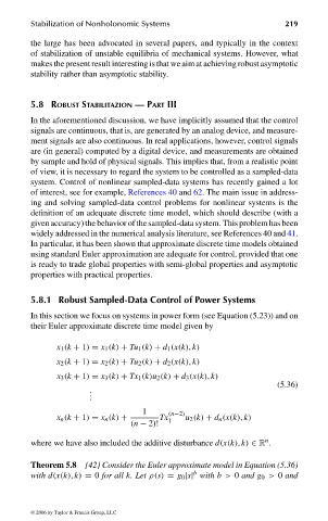
In this section we focus on systems in power form (see Equation (5.23)) and on
their Euler approximate discrete time model given by

x 1 (k + 1) = x 1 (k) + Tu 1 (k) + d 1 (x(k), k)
x 2 (k + 1) = x 2 (k) + Tu 2 (k) + d 2 (x(k), k)

x 3 (k + 1) = x 3 (k) + Tx 1 (k)u 2 (k) + d 3 (x(k), k)
(5.36)
.
.
.
1 (n−2)
x n (k + 1) = x n (k) + Tx 1 u 2 (k) + d n (x(k), k)
(n − 2)!
n
where we have also included the additive disturbance d(x(k), k) ∈ R .
Theorem 5.8 [42] Consider the Euler approximate model in Equation (5.36)
b
with d(x(k), k) = 0 for all k. Let ρ(s) = g 0 |s| with b > 0 and g 0 > 0 and

© 2006 by Taylor & Francis Group, LLC

FRANKL: “dk6033_c005” — 2006/3/31 — 16:42 — page 219 — #33