Page 272 - Autonomous Mobile Robots

258 Autonomous Mobile Robots

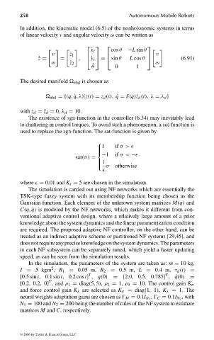
In addition, the kinematic model (6.5) of the nonholonomic systems in terms
of linear velocity v and angular velocity ω can be written as

   
˙ x c cos θ −L sin θ
v ˙ z 1 v
 

˙ z = = , ˙y c = sin θ  (6.91)
ω ˙ z 2 L cos θ  ω
˙ θ 0 1
The desired manifold nhd is chosen as

nhd ={(q, ˙q, λ)|z(t) = z d (t), ˙q = S(q)˙z d (t), λ = λ d }

with z d =˙z d = 0, λ d = 10.
The existence of sgn-function in the controller (6.34) may inevitably lead
to chattering in control torques. To avoid such a phenomenon, a sat-function is
used to replace the sgn-function. The sat-function is given by

1 if σ>




−1 if σ< −
sat(σ) =
1

σ otherwise


where = 0.01 and K s = 5 are chosen in the simulation.
The simulation is carried out using NF networks which are essentially the
TSK-type fuzzy system with its membership function being chosen as the
Gaussian function. Each element of the unknown system matrices M(q) and
C(q, ˙q) is modeled by the NF networks, which makes it different from con-
ventional adaptive control design, where a relatively large amount of a prior
knowledge about the system dynamics and the linear parametrization condition
are required. The proposed adaptive NF controller, on the other hand, can be
treated as an indirect adaptive scheme or partitioned NF systems [29,45], and
doesnotrequireanypreciseknowledgeonthesystemdynamics. Theparameters
in each NF subsystem can be separately tuned, which yield a faster updating
speed, as can be seen from the simulation results.
In the simulation, the parameters of the system are taken as: m = 10 kg,
2
I = 5 kgm , R 1 = 0.05 m, R 2 = 0.5 m, L = 0.4 m, τ d (t) =
T T
[0.5 sin t, 0.1 sin t, 0.2 cos t] , q(0) =[2.0, 0.5, 0.785] , ˙q(0) =
T
[0.2, 0.2, 0] , and ρ 1 = diag(5, 5), ρ 2 = 1, ρ 3 = 10. The control gain K σ
and force control gain K λ are selected as K σ = diag(1, 1), K λ = 1. The
, with
neural weights adaptation gains are chosen as M = 0.1I N 1 , C = 0.1I N 2
N 1 = 100 and N 2 = 200 being the number of rules of the NF system to estimate
matrices M and C, respectively.

© 2006 by Taylor & Francis Group, LLC

FRANKL: “dk6033_c006” — 2006/3/31 — 16:42 — page 258 — #30