Page 121 - Autonomous Mobile Robots

104 Autonomous Mobile Robots

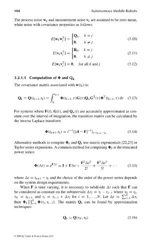
The process noise w k and measurement noise v k are assumed to be zero-mean,
white noise with covariance properties as follows:

Q k , k = j
T
E[w k w ]= (3.10)
j
0, k = j

R k , k = j
T
E[v k v ]= (3.11)
j
0, k = j
T
E[w k v ]= 0, for all k and j (3.12)
j
3.2.1.1 Computation of and Q k
The covariance matrix associated with w(t k ) is:

t k+1

T T
Q k = Q(t k+1 , t k ) = (t k+1 , τ)G(τ)Q w G (τ) (t k+1 , τ) dτ (3.13)
t k
For systems where F(t), G(t), and Q w (t) are accurately approximated as con-
stant over the interval of integration, the transition matrix can be calculated by
the inverse Laplace transform

(t k+1 , t k ) = −1 {[sI − F] −1 } t=t k+1 −t k (3.14)

Alternative methods to compute k and Q k use matrix exponentials [22,23] or
Taylor series expansions. A common method for computing k is the truncated
power series:

2
3
F t 2 F t 3
F t
( t) = e = I + F t + + + ··· (3.15)
2! 3!
where t = t k+1 − t k and the choice of the order of the power series depends
on the system design requirements.
When F is time varying, it is necessary to subdivide t such that F can
be considered as constant on the subintervals τ i = τ i − τ i−1 where τ 0 = t k ,
N

τ N = t k+1 , and τ i = τ i−1 + τ i for i = 1, ... , N. Let t = τ i
i=1
N
then k i=1 (τ i , τ i−1 ). The matrix Q k can be found by approximation
techniques:
Q k = Q(τ N , τ 0 ) (3.16)

© 2006 by Taylor & Francis Group, LLC

FRANKL: “dk6033_c003” — 2006/3/31 — 16:42 — page 104 — #6