Page 124 - Autonomous Mobile Robots

Data Fusion via Kalman Filter 107

assumption is that we have a model available, of the form of Equation (3.8)
and Equation (3.9), suitable for accurate propagation of the state estimate and
state estimate error covariance matrix between measurement instants. Second,
Step 3 is the only step that requires the measurement; therefore, when the next
measurement time can be accurately predicted, then Steps 1 and 2 are often com-
puted prior to the arrival of the next measurement. The purpose of doing this is
to minimize the computational delay between the arrival of y k and availability
of ˆ x k|k to the other online processes that need it (e.g., planning, guidance, or
control). Third, the portions of the KF algorithm that require the majority of the
computations are Equation (3.22), Equation (3.23), and Equation (3.25), which
are related to maintaining the error covariance matrix and the Kalman gain.

3.2.2.1 Implementation issues
The performance of the KF depends on the accuracy of the process model
and the measurement model. The implementation approach also affects the
performance and computational load of the KF. This section discusses some of
the important implementation issues related to the KF.

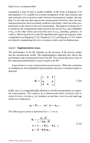
Sequential processing of independent measurements. When the system has
m simultaneous, but independent measurements, the noise covariance matrix is
diagonal:

 
r 1 0 0
.
 .  (3.26)
0 . 0 
R k = 
0 0 r m
In this case, it is computationally efficient to treat the measurements as sequen-
tial measurements. This replaces an m-dimensional matrix inversion with m
scalar divisions. At time t k , we introduce an auxiliary vector ˆ x 0 and matrix p 0
which are initialized as

p 0 = P k|k−1 and ˆ x 0 = ˆ x k|k−1 (3.27)

The following recursion is performed for i = 1to m:

p i−1 h i T
K i =
r i + h i p i−1 h T
i
(3.28)
ˆ x i = ˆ x i−1 + K i [y i − h i ˆ x i−1 ]
p i =[I − K i h i ]p i−1

© 2006 by Taylor & Francis Group, LLC

FRANKL: “dk6033_c003” — 2006/3/31 — 16:42 — page 107 — #9