Page 123 - Autonomous Mobile Robots

106 Autonomous Mobile Robots

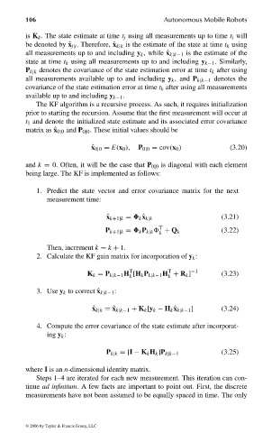
is K k . The state estimate at time t j using all measurements up to time t i will
be denoted by ˆ x j|i . Therefore, ˆ x k|k is the estimate of the state at time t k using
all measurements up to and including y k , while ˆ x k|k−1 is the estimate of the
state at time t k using all measurements up to and including y k−1 . Similarly,
P k|k denotes the covariance of the state estimation error at time t k after using
all measurements available up to and including y k , and P k|k−1 denotes the
covariance of the state estimation error at time t k after using all measurements
available up to and including y k−1 .
The KF algorithm is a recursive process. As such, it requires initialization
prior to starting the recursion. Assume that the first measurement will occur at
t 1 and denote the initialized state estimate and its associated error covariance
matrix as ˆ x 0|0 and P 0|0 . These initial values should be

ˆ x 0|0 = E(x 0 ), P 0|0 = cov(x 0 ) (3.20)

and k = 0. Often, it will be the case that P 0|0 is diagonal with each element
being large. The KF is implemented as follows:

1. Predict the state vector and error covariance matrix for the next
measurement time:

(3.21)
ˆ x k+1|k = k ˆ x k|k
T
P k+1|k = k P k|k + Q k (3.22)
k
Then, increment k = k + 1.
2. Calculate the KF gain matrix for incorporation of y k :
T T −1
K k = P k|k−1 H [H k P k|k−1 H + R k ] (3.23)
k
k
3. Use y k to correct ˆ x k|k−1 :

ˆ x k|k = ˆ x k|k−1 + K k [y k − H k ˆ x k|k−1 ] (3.24)

4. Compute the error covariance of the state estimate after incorporat-
ing y k :

P k|k =[I − K k H k ]P k|k−1 (3.25)

where I is an n-dimensional identity matrix.
Steps 1–4 are iterated for each new measurement. This iteration can con-
tinue ad infinitum. A few facts are important to point out. First, the discrete
measurements have not been assumed to be equally spaced in time. The only

© 2006 by Taylor & Francis Group, LLC

FRANKL: “dk6033_c003” — 2006/3/31 — 16:42 — page 106 — #8