Page 153 - Autonomous Mobile Robots
P. 153

136                                    Autonomous Mobile Robots


                                                                x –
                                         Du, Dv     INS                                x
                                   IMU
                                                  equations                     +   +    Position
                                                                                         velocity
                                       Ephemeris
                                                           Measurement             dx    attitude
                                                            prediction
                                                                Predicted measurements
                                           Measurements          –  Residuals
                                    GPS                                        Kalman filter
                                                            +

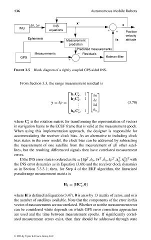
                                FIGURE 3.5 Block diagram of a tightly coupled GPS aided INS.


                                   From Section 3.3, the range measurement residual is

                                                                e   
                                                             h 1 C ,  1    
                                                                 n      δn
                                                                 e
                                                             h 2 C ,
                                                                      δe
                                                                 n  1    
                                                                    
                                                            
                                                                 .                      (3.70)
                                                                 .
                                                   y = δρ =         
                                                                       
                                                                .    δd 
                                                                 e
                                                             h m C ,1   b u
                                                                 n
                                       e
                                where C is the rotation matrix for transforming the representation of vectors
                                       n
                                in navigation frame to the ECEF frame that is valid at the measurement epoch.
                                When using this implementation approach, the designer is responsible for
                                accommodating the receiver clock bias. As an alternative to including clock
                                bias states in the error model, the clock bias can be addressed by subtracting
                                the measurement of one satellite from the measurement of all other satel-
                                lites, but the resulting differenced signals then have correlated measurement
                                errors.
                                                                                     T
                                                                                        T T
                                                                     T
                                                                                  T
                                                                            T ˙
                                   If the INS error state is ordered as δx =[δp , b u , δv , b u , δρ , x , x ] with
                                                                                     a  g
                                the INS error dynamics as in Equation (3.68) and the receiver clock dynamics
                                as in Section 3.3.3.1; then, for Step 4 of the EKF algorithm, the linearized
                                pseudorange measurement matrix is
                                                                  e
                                                          H k =[HC , 0]
                                                                  n
                                where H is defined in Equation (3.47), 0 is an m by 13 matrix of zeros, and m is
                                the number of satellites available. Note that the components of the error in this
                                vector of measurements are uncorrelated. Whether or not the measurement error
                                can be considered white depends on which GPS error correction approaches
                                are used and the time between measurement epochs. If significantly correl-
                                ated measurement errors exist, then they should be addressed through state
                                 © 2006 by Taylor & Francis Group, LLC


                                FRANKL: “dk6033_c003” — 2006/3/31 — 16:42 — page 136 — #38
   148   149   150   151   152   153   154   155   156   157   158