Page 157 - Autonomous Mobile Robots

140 Autonomous Mobile Robots

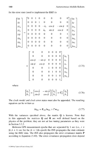
for the error state (used to implement the EKF) is

 
δ˙n δn
  0 0 1 0 0 0 0 0  
0 0 0 1 0 0 0 

   
 δ˙e  0 δe 

 
   
 0 0 0 0 cos ψ − sin ψ 
 δv n
 δ˙v n  −ˆa e 0  

     
  0 0 0 0 ˆ a n sin ψ cos ψ 0  
δ˙v e  δv e 
 
   
0 0 0 0 0 0 0 
= 
   
δ ˙ ψ  1 δψ 

 
   
 0 0 0 0 0 0 0 
 δa u
  0  

δ˙a u 
    
  0 0 0 0 0 0 0 0  
δ˙a v  δa v 
 
0 0 0 0 0 0 0 0
δ ˙ω r δω r
0 0 0 0 0 0
 
 0 0 0 0 0 0  n u 



   

 cos ψ − sin ψ 0 0 0 0 n v 
 
 
sin ψ cos ψ 0 0 0  
 

0 n r 
+     (3.75)
 0 0 1 0 0   


0  n b 1 
   
 0 0 0 1 0 
 0 n b 2 

 
 0 0 0 0 1 0 n b 3
0 0 0 0 0 1
where

ˆ a n cos ˆ ψ − sin ˆ ψ ˜ a u ˆ n ˆa u
= = C b (3.76)
ˆ a e sin ˆ ψ cos ˆ ψ ˜ a v ˆ a v
The clock model and clock error states must also be appended. The resulting
equation can be written as
δ˙ x ins = F ins δx ins + w ins (3.77)
With the variances specified above, the matrix Q is known. Note that
in this approach the matrices Q and R are well defined based on the
physics of the problem; they are not ad hoc tuning parameters as they were
in Section 3.3.3.
Between GPS measurement epochs that are separated by 1 sec (i.e., t ∈
[k, k + 1) sec for the (k + 1)th epoch) the INS propagates the state estimate
using the IMU data. The INS also propagates the error covariance matrix P
according to Equation (3.40). The error covariance propagation does depend
© 2006 by Taylor & Francis Group, LLC
FRANKL: “dk6033_c003” — 2006/3/31 — 16:42 — page 140 — #42