Page 154 - Autonomous Mobile Robots
P. 154
Data Fusion via Kalman Filter 137
augmentation and possibly a Schmidt–Kalman filter implementation approach
[19,20].
As opposed to a loosely coupled system, the designer of a tightly coupled
system must implement ephemeris calculations, implement a receiver clock
model, and be familiar with various receiver specific issues and peculiarit-
ies. The payoff for this increased level of understanding is potentially better
performance. The higher performance is achievable because the various meas-
urement errors and their covariance can be properly modeled and incorporated
in the design approach. As in the loosely coupled approach, the tightly
coupled approach does attempt to estimate IMU calibration parameters (e.g.,
biases). As the errors are calibrated, the rate of growth of the INS errors will
decrease.
Example 3.6 This example uses the same hypothetical 2D world as in
Example 3.4. Simulation results are shown in Figure 3.6. The vehicle traject-
ory is also similar to that in the previous example. In this example, using GPS
measurement epochs that have 1 sec duration, at the (k + 1)th measurement
epoch (i.e., t = k + 1) the GPS range vector will be used as measurements in
the EKF to estimate the INS error state. The GPS measurements are computed
as the actual range plus a linearly increasing clock bias, and Gaussian ran-
dom noise with unit variance. In addition to the GPS receiver, the vehicle
is equipped with an IMU and a computer capable of integrating the INS
equations.
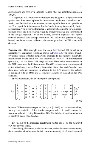
In two dimensions, the INS integrates the equation
˙ ˆ n 0 0 1 0 0 0 0 0
ˆ n
ˆ e 0 0 0 1 0 ˆe 0
˙ 0
0 ˜ a u
˙
˙
ˆ x = ˆv n = 0 0 0 0 0 ˆv n + cos ˆ ψ − sin ˆ ψ 0 ˜a v
˙ 0 0 0 0 0 ˆv e ω r
˜
ˆv e sin ˆ ψ cos ˆ ψ 0
˙ ˆ ψ 0 0 0 0 0 ˆ ψ 0 0 1
(3.71)
between GPS measurement epochs, that is, t ∈[k, k+1) sec. In these equations,
for a generic variable z, ˆz denotes the computed value of z and ˆz denotes the
measured value of z. Using this notation, [δˆa u , δˆa v , δ ˆω r ] are the estimated values
of the IMU biases [δa u , δa v , δω r ].
Let (˜a u , ˜a v ) be the measured acceleration vector and ˜ω r be the measured
yaw rate in body frame.
Considering bias errors, scale factor errors, and white measurement noise,
the assumed relationsbetween the IMU measurements(˜a u , ˜a v , ˜ω r )andtheactual
© 2006 by Taylor & Francis Group, LLC
FRANKL: “dk6033_c003” — 2006/3/31 — 16:42 — page 137 — #39

