Page 318 - Autonomous Mobile Robots

306 Autonomous Mobile Robots

Then the system (8.22) becomes

˙ ˜ η = Q( ˜γ)µ = Q( ˜γ)E −1 ( ˜γ)R( ˜ θ) v d = (˜η, v d ) (8.25)
¯
0

˙
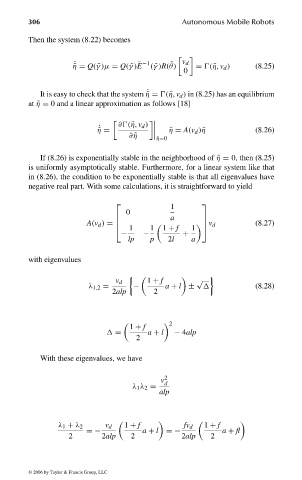
It is easy to check that the system ˜η = (˜η, v d ) in (8.25) has an equilibrium
at ˜η = 0 and a linear approximation as follows [18]

∂ (˜η, v d )
˙
˜ η = ˜ η = A(v d )˜η (8.26)
∂ ˜η
˜ η=0
If (8.26) is exponentially stable in the neighborhood of ˜η = 0, then (8.25)
is uniformly asymptotically stable. Furthermore, for a linear system like that
in (8.26), the condition to be exponentially stable is that all eigenvalues have
negative real part. With some calculations, it is straightforward to yield

1
 
0
a
 
A(v d ) = 
 v d (8.27)
 1 1 1 + f 1 
− − +
lp p 2l a
with eigenvalues

√
v d 1 + f
λ 1,2 = − a + l ± (8.28)
2alp 2

1 + f

2
= a + l − 4alp
2
With these eigenvalues, we have

v 2 d
λ 1 λ 2 =
alp

λ 1 + λ 2 v d 1 + f fv d 1 + f
=− a + l =− a + fl
2 2alp 2 2alp 2

© 2006 by Taylor & Francis Group, LLC

FRANKL: “dk6033_c008” — 2006/3/31 — 16:43 — page 306 — #12