Page 323 - Autonomous Mobile Robots

Unified Control Design for Autonomous Vehicle 311

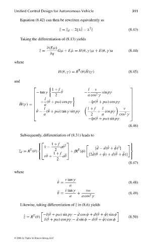
Equation (8.42) can then be rewritten equivalently as

2
˙
¨ z =¨z d − 2ξλ˜z − λ ˜z (8.43)
Taking the differentiation of (8.13) yields

∂(Eµ)
¨ z = Gµ + E ˙µ = H(θ, γ)µ + E(θ, γ)u (8.44)
∂q
where

T
H(θ, γ) = R (θ)H(γ ) (8.45)
¯
and

 
1 + f l v
− tan γ ˙ θ − sin pγ
2 a cos γ
 2 
 
l
 
 + ( ˙ θ + pω) cos pγ −lp( ˙ θ + pω) cos pγ 
¯
H(γ ) =  a 


l 1 + f l v
 
 ˙ θ − ( ˙ θ + pω) tan γ sin pγ + cos pγ 
2
 a 2 a cos γ 
−lp( ˙ θ + pω) sin pγ
(8.46)
Subsequently, differentiation of (8.31) leads to
1 + f 2
  
 ˙v − a ˙ θ ¨ 2 


T  2  + fR (φ) {d − d( ˙ θ + ˙ φ) }
T

1 + f ˙
¨ z d = R (θ) 
 {2d( ˙ θ + ˙ φ) + d( ¨ θ + ¨ φ)} 
v ˙ θ + a ¨ θ
 
2
(8.47)
where
v tan γ
˙ θ = (8.48)
a
˙ v tan γ vω
¨ θ = + (8.49)
2
a a cos γ
Likewise, taking differentiation of ˜z in (8.6) yields
˙
T
˙ ˜ z = R (θ) −l( ˙ θ + pω) sin pγ − d cos φ + d( ˙ θ + ˙ φ) sin φ (8.50)
l( ˙ θ + pω) cos pγ − d sin φ − d( ˙ θ + ˙ φ) cos φ
˙
© 2006 by Taylor & Francis Group, LLC

FRANKL: “dk6033_c008” — 2006/3/31 — 16:43 — page 311 — #17