Page 14 - Basic Structured Grid Generation

Mathematical preliminaries – vector and tensor analysis 3

Given the set {g 1 , g 2 , g 3 } we can form the set of contravariant base vectors at P,
2
1
3
{g , g , g }, defined by the set of scalar product identities
i
g · g j = δ i (1.6)
j
i
where δ is the Kronecker symbol given by
j

1 when i = j
i
δ = (1.7)
j 0 when i = j
i
Exercise 1. Deduce from the definitions (1.6) that the g s may be expressed in terms
of vector products as
1 g 2 × g 3 2 g 3 × g 1 3 g 1 × g 2
g = , g = , g = (1.8)
V V V
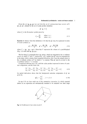
where V ={g 1 · (g 2 × g 3 )}. (Note that V represents the volume of a parallelepiped
(Fig. 1.2) with sides g 1 , g 2 , g 3 .)

1
The fact that g is perpendicular to g 2 and g 3 , which are tangential to the co-ordinate
1
3
2
curves on which x and x , respectively, vary, implies that g must be perpendicular
to the plane which contains these tangential directions; this is just the tangent plane to
1
i
the co-ordinate surface at P on which x is constant. Thus g must be normal to the
i
co-ordinate surface x = constant.
Comparison between eqn (1.6), with the scalar product expressed in terms of carte-
sian components, and the chain rule
∂x i ∂y 1 ∂x i ∂y 2 ∂x i ∂y 3 ∂x i ∂y k ∂x i i
+ + = = = δ j (1.9)
∂y 1 ∂x j ∂y 2 ∂x j ∂y 3 ∂x j ∂y k ∂x j ∂x j
i
for partial derivatives shows that the background cartesian components of g are
given by
∂x i
i
(g ) j = , j = 1, 2, 3. (1.10)
∂y j
In eqn (1.9) we have made use of the summation convention, by which repeated
indices in an expression are automatically assumed to be summed over their range

g 2
g 3
V

P
g 1

Fig. 1.2 Parallelepiped of base vectors at point P.