Page 16 - Basic Structured Grid Generation

Mathematical preliminaries – vector and tensor analysis 5

g 23 = g 32 = x η x ς + y η y ς + z η z ς
g 31 = g 13 = x ς x ξ + y ς y ξ + z ς z ξ

where a typical partial derivative ∂x has been written as x ξ , and the superscript 2 now
∂ξ
represents squaring.
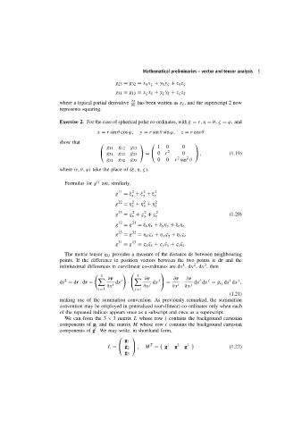
Exercise 2. For the case of spherical polar co-ordinates, with ξ = r, η = θ, ς = ϕ,and

x = r sin θ cos ϕ, y = r sin θ sin ϕ, z = r cos θ
show that
   
1 0 0
g 11 g 12 g 13
 g 21 g 22 g 23  =  0 r 2 0  , (1.19)
2
2
g 31 g 32 g 33 0 0 r sin θ
where (r, θ, ϕ) take the place of (ξ, η, ς).
Formulas for g ij are, similarly,

11 2 2 2
g = ξ + ξ + ξ z
y
x
2
2
g 22 = η + η + η 2 z
y
x
2
2
g 33 = ς + ς + ς 2 (1.20)
x y z
12 21
g = g = ξ x η x + ξ y η y + ξ z η z
23 32
g = g = η x ς x + η y ς y + η z ς z
31 13
g = g = ς x ξ x + ς y ξ y + ς z ξ z .
Themetrictensor g ij provides a measure of the distance ds between neighbouring
points. If the difference in position vectors between the two points is dr and the
3
1
2
infinitesimal differences in curvilinear co-ordinates are dx ,dx ,dx ,then
 
3 3

2 ∂r i ∂r j ∂r ∂r i j i j
ds = dr · dr = dx ·  dx  = · dx dx = g ij dx dx ,
∂x i ∂x j ∂x i ∂x j
i=1 j=1
(1.21)
making use of the summation convention. As previously remarked, the summation
convention may be employed in generalized (curvilinear) co-ordinates only when each
of the repeated indices appears once as a subscript and once as a superscript.
We can form the 3 × 3matrix L whose row i contains the background cartesian
components of g i and the matrix M whose row i contains the background cartesian
i
components of g . We may write, in shorthand form,
 
g 1
T
L =  g 2  , M = g 1 g 2 g 3 (1.22)
g 3