Page 198 - Basic Structured Grid Generation

Moving grids and time-dependent co-ordinate systems 187

7.5 Application to a moving boundary problem

The ‘in-cylinder’ calculation for an internal combustion engine gives us an application
of a time-dependent co-ordinate system. The physical domain in this case is the volume
between cylinder head and piston face. The piston moves between the B.D.C. (bottom
dead centre) position and the T.D.C. (top dead centre) position, and so the physical
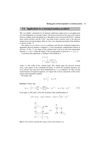
domain has a moving boundary. Here we take a two-dimensional model of the situation,
as shown in Fig. 7.1.
Our objective is to obtain a set of co-ordinates such that the irregularly-shaped time-
dependent physical domain is mapped to a fixed rectangular computational domain at
all times. In Fig. 7.1 the shape of the cylinder head is given by the time-independent
function y = y b (x), while the shape of the moving piston is given by y = y a (x, t).
A possible time-dependent co-ordinate transformation is

ξ = x/l
y − y a (x, t)
η = . (7.40)
y b (x) − y a (x, t)
where l is the width of the cylinder head. This clearly maps the physical domain
onto a unit square in the computational plane, in which the transport equations are
to be solved, once they have been transformed to ξ, η co-ordinates. To carry out the
transformation of transport equations, we require the various components of the metric
tensors and Christoffel symbols.
We begin with
1
ξ x = , ξ y = 0.
l
Exercise 3. Show that

∂y a dy b −1 −1
η x =− (1 − η) + η (y b − y a ) , η y = (y b − y a ) . (7.41)
∂x dx
From eqns (1.160) and (1.162) the Jacobian of the transformation is
√ g −1
g = x ξ y η − x η y ξ = g(ξ x η y − ξ y η x ) = (y b − y a ) .
l

y
h
y =y (x)
b
D C 1
D C
A B
y =y (x,t) 0 A B
a
1 x
0
L x
Fig. 7.1 Piston-cylinder assembly with irregular cylinder head and piston face.