Page 100 - Biomedical Engineering and Design Handbook Volume 1, Fundamentals

PHYSICAL AND FLOW PROPERTIES OF BLOOD 77

Insertion of Eq. (3.21) into (3.20) yields the Bessel equation,
2
3
dW + 1 dW + i ωρ W = − A
dr 2 r dr μ μ (3.22)
The solution for Eq. (3.22) is
⎧ ⎛ ω / 32 ⎞ ⎫
⎪ J 0 ⎜ r • i ⎟ ⎪
K 1 ⎪ ⎝ v ⎠ ⎪
Wr () = 1 ⎨ − ⎬ (3.23)
ρω ⎪ ⎛ ω / 32 ⎪
⎞
i
⎪ J 0 ⎜ ⎝ R v • i ⎟ ⎟ ⎠ ⎪
⎩ ⎭
where J is a Bessel function of order zero of the first kind, v = m/r is the kinematic viscosity, and a
0
is a dimensionless parameter known as the Womersley number and given by
ω
α = R 0 (3.24)
v
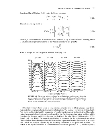
When a is large, the velocity profile becomes blunt (Fig. 3.6).

FIGURE 3.6 Theoretical velocity profiles of an oscillating flow resulting from a sinusoidal
pressure gradient (cos w t) in a pipe. a is the Womersley number. Profiles are plotted for intervals
of Δw t = 15°. For w t > 180°, the velocity profiles are of the same form but opposite in sign.
[From Nichols and O’Rourke (1998) by permission.]

Pulsatile flow in an elastic vessel is very complex, since the tube is able to undergo local defor-
mations in both longitudinal and circumferential directions. The unsteady component of the pulsatile
flow is assumed to be induced by propagation of small waves in a pressurized elastic tube. The mathe-
matical approach is based on the classical model for the fluid-structure interaction problem, which
describes the dynamic equilibrium between the fluid and the tube thin wall (Womersley, 1955b;
Atabek and Lew, 1966). The dynamic equilibrium is expressed by the hydrodynamic equations
(Navier-Stokes) for the incompressible fluid flow and the equations of motion for the wall of an elastic
tube, which are coupled together by the boundary conditions at the fluid-wall interface. The
ˆ z
ˆ r
motion of the liquid is described in a fixed laboratory coordinate system ( , q, ), and the dynamic