Page 421 - Biomimetics : Biologically Inspired Technologies

Bar-Cohen : Biomimetics: Biologically Inspired Technologies DK3163_c016 Final Proof page 407 21.9.2005 11:49pm

Biomimetic and Biologically Inspired Control 407

constraints considered in some of these approaches may not really be applied by the biological
system. There are also several drawbacks such as: (1) all approaches need numerous computation
of the Jacobian matrix and/or its pseudo-inverse; (2) the approaches 2 and 3 may be numerically
unstable; and (3) the so-called quasicyclic problem (Lee and Kil, 1994). Therefore, research
on how the biological system organizes its sensory-motor coordination should reflect not only
the mathematical aspects of the algorithm and its computational efficiency, but also the bio-
logical reality.

16.2.3.2 Diffusion-Based Learning Algorithm

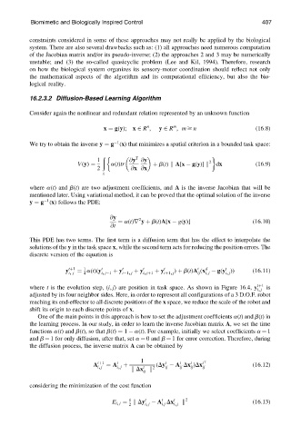
Consider again the nonlinear and redundant relation represented by an unknown function

n
m
x ¼ g(y); x 2 R , y 2 R , m $ n (16:8)
1
We try to obtain the inverse y ¼ g (x) that minimizes a spatial criterion in a bounded task space:
ð
T
1 @y @y
V(y) ¼ a(t)tr þ b(t) k A[x g(y)] k 2 dx (16:9)
2 @x @x
x
where a(t) and b(t) are two adjustment coefficients, and A is the inverse Jacobian that will be
mentioned later. Using variational method, it can be proved that the optimal solution of the inverse
1
y ¼ g (x) follows the PDE:

@y 2
¼ a(t)r y þ b(t)A[x g(y)] (16:10)
@t
This PDE has two terms. The first term is a diffusion term that has the effect to interpolate the
solutions of the y in the task space x, while the second term acts for reducing the position errors. The
discrete version of the equation is

t
d
t
1
y tþ1 ¼ a(t)(y t i, j 1 þ y t i 1, j þ y t i, jþ1 þ y t iþ1, j ) þ b(t)A (x g(y )) (16:11)
i; j
ij
4
i, j
i, j
where t is the evolution step, (i, j) are position in task space. As shown in Figure 16.4, y tþ1 is
i, j
adjusted by its four neighbor sides. Here, in order to represent all configurations of a 3 D.O.F. robot
reaching its end-effector to all discrete positions of the x space, we reduce the scale of the robot and
shift its origin to each discrete points of x.
One of the main points in this approach is how to set the adjustment coefficients a(t) and b(t)in
the learning process. In our study, in order to learn the inverse Jacobian matrix A, we set the time
functions a(t) and b(t), so that b(t) ¼ 1 a(t). For example, initially we select coefficients a ¼ 1
and b ¼ 1 for only diffusion, after that, set a ¼ 0 and b ¼ 1 for error correction. Therefore, during
the diffusion process, the inverse matrix A can be obtained by
1 t t t t T
t
tþ1
A ¼ A þ (Dy A Dx )Dx (16:12)
i, j i, j t 2 ij ij ij ij
k Dx ij k
considering the minimization of the cost function
t
1
E i, j ¼ k Dy t A Dx t k 2 (16:13)
2 i, j i:j i, j