Page 422 - Biomimetics : Biologically Inspired Technologies

Bar-Cohen : Biomimetics: Biologically Inspired Technologies DK3163_c016 Final Proof page 408 21.9.2005 11:49pm

408 Biomimetics: Biologically Inspired Technologies

(i,j + 1)
(i,j + 1)
(i + 1,j)
(i − 1,j)
(i − 1,j) (i + 1,j)
(i,j)
(i,j)
(i,j − 1)
(i,j − 1)

Origin

Origin
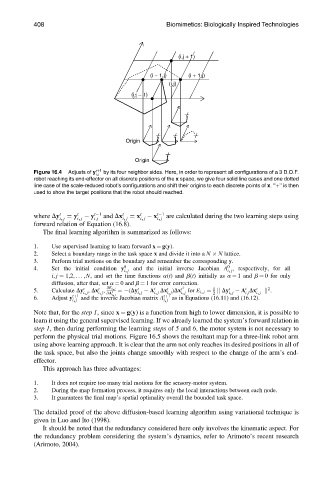
Figure 16.4 Adjusts of y tþ1 by its four neighbor sides. Here, in order to represent all configurations of a 3 D.O.F.
i,j
robot reaching its end-effector on all discrete positions of the x space, we give four solid line cases and one dotted
line case of the scale-reduced robot’s configurations and shift their origins to each discrete points of x.‘‘þ’’ is then
used to show the target positions that the robot should reached.

where Dy t i, j ¼ y t i, j y t 1 and Dx t i, j ¼ x t i, j x t 1 are calculated during the two learning steps using
i:j
i, j
forward relation of Equation (16.8).
The final learning algorithm is summarized as follows:
1. Use supervised learning to learn forward x ¼ g(y).
2. Select a boundary range in the task space x and divide it into a N N lattice.
3. Perform trial motions on the boundary and remember the corresponding y.
0
4. Set the initial condition y 0 and the initial inverse Jacobian A , respectively, for all
i, j i, j
i, j ¼ 1,2, .. . , N, and set the time functions a(t) and b(t) initially as a ¼ 1 and b ¼ 0 for only
diffusion, after that, set a ¼ 0 and b ¼ 1 for error correction.
t
t
T
2
t
t
1
t
t ¼ (Dy
5. Calculate Dy , Dx , @E i, j t i, j A Dx )Dx t i, j for E i, j ¼ k Dy t i, j A Dx t i, j k .
i, j
i:j
i, j
i, j
2
i, j @A i, j
6. Adjust y tþ1 and the inverse Jacobian matrix A tþ1 as in Equations (16.11) and (16.12).
i, j i, j
Note that, for the step 1, since x ¼ g(y) is a function from high to lower dimension, it is possible to
learn it using the general supervised learning. If we already learned the system’s forward relation in
step 1, then during performing the learning steps of 5 and 6, the motor system is not necessary to
perform the physical trial motions. Figure 16.5 shows the resultant map for a three-link robot arm
using above learning approach. It is clear that the arm not only reaches its desired positions in all of
the task space, but also the joints change smoothly with respect to the change of the arm’s end-
effector.
This approach has three advantages:
1. It does not require too many trial motions for the sensory-motor system.
2. During the map formation process, it requires only the local interactions between each node.
3. It guarantees the final map’s spatial optimality overall the bounded task space.
The detailed proof of the above diffusion-based learning algorithm using variational technique is
given in Luo and Ito (1998).
It should be noted that the redundancy considered here only involves the kinematic aspect. For
the redundancy problem considering the system’s dynamics, refer to Arimoto’s recent research
(Arimoto, 2004).