Page 118 - Buried Pipe Design

Design of Gravity Flow Pipes 93

the hyperbolic soil model 6,42,43 provides a nonlinear soil model that has
been used successfully in finite element analyses of buried pipe. Thus,
the hyperbolic model is incorporated in most finite element programs
that are used in buried pipe analysis. Examples are CANDE and
PIPE5.
The Iowa formula, as proposed by Spangler, predicted the change
in the horizontal diameter of the pipe due to soil placed over the top
56
of the pipe. Watkins and Spangler proposed the use of the modulus
of soil reaction E with units of force per length squared. Later
Watkins, Spangler, and others showed that the vertical and horizon-
tal deflections were about equal for small deflection. They also
showed that the vertical deflection was the better predictor relating
to pipe performance. While the Iowa formula has been criticized by
some, it remains the best known simplified method for computing
deflections.
Howard’s E values (Table 3.4), back-calculated from measured
vertical deflections of many flexible pipe installations, are conserv-
ative. For the back-calculation, he had to assume the bedding factor
and the lag factor. Some have proposed an increasing soil modulus
with depth of cover, but Howard found no correlation between E
and depth of fill. His data were limited to 50 ft of cover, so he stated
that his proposed values of E may not be valid for cover greater
than 50 ft.
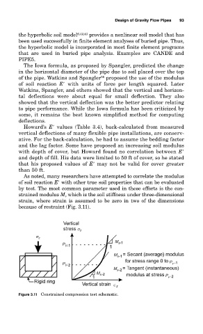
As noted, many researchers have attempted to correlate the modulus
of soil reaction E with other true soil properties that can be evaluated
by test. The most common parameter used in these efforts is the con-
strained modulus M s which is the soil stiffness under three-dimensional
strain, where strain is assumed to be zero in two of the dimensions
because of restraint (Fig. 3.11).

s z
s z
M
P V s
M s
P
P V v
M s
M s P v

Πz
Figure 3.11 Constrained compression test schematic.