Page 117 - Calculus Demystified

CHAPTER 4
The Integral
104
the set P a partition. Sometimes, to be more specific, we call it a uniform partition
(to indicate that all the subintervals have the same length). Refer to Fig. 4.3.
_
b a
k
x 0 = a x j x k = b
Fig. 4.3

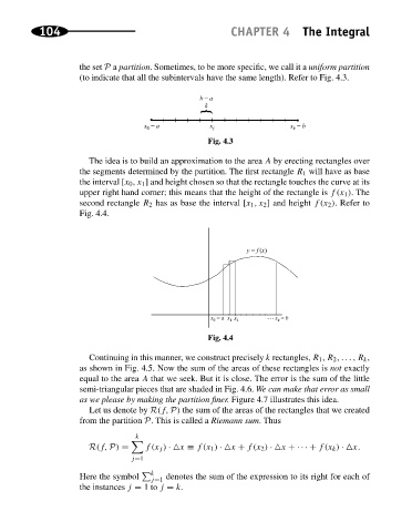
The idea is to build an approximation to the area A by erecting rectangles over
the segments determined by the partition. The first rectangle R 1 will have as base
the interval [x 0 ,x 1 ] and height chosen so that the rectangle touches the curve at its
upper right hand corner; this means that the height of the rectangle is f(x 1 ). The
second rectangle R 2 has as base the interval [x 1 ,x 2 ] and height f(x 2 ). Refer to
Fig. 4.4.

y = f (x)

x 0 = a x 1 x 2 x k = b
Fig. 4.4

Continuing in this manner, we construct precisely k rectangles, R 1 ,R 2 ,...,R k ,
as shown in Fig. 4.5. Now the sum of the areas of these rectangles is not exactly
equal to the area A that we seek. But it is close. The error is the sum of the little
semi-triangular pieces that are shaded in Fig. 4.6. We can make that error as small
as we please by making the partition finer. Figure 4.7 illustrates this idea.
Let us denote by R(f, P) the sum of the areas of the rectangles that we created
from the partition P. This is called a Riemann sum. Thus

k

R(f, P) = f(x j ) · x ≡ f(x 1 ) · x + f(x 2 ) · x + ··· + f(x k ) · x.
j=1

k
Here the symbol j=1 denotes the sum of the expression to its right for each of
the instances j = 1to j = k.