Page 426 - Cam Design Handbook

THB13 9/19/03 7:56 PM Page 414

414 CAM DESIGN HANDBOOK

m Ê a cos ( nT)+ b sin ( nT) ˆ
X = Â Á n n ˜. (13.27)
2
F
2 Ë F - n 2 ¯
2
n=0 2
The required integration of Eq. (13.22) and Eq. (13.25) can now be performed exactly.
The 2m + 1 coefficients can then be determined from the two equations, Eq. (13.23), and
the 2m + 1 - 2l extremum conditions
dP dP dP
= = = 0, i 1= ◊◊◊, , ml (13.28)
- .
da da db
0 i i
Using this approach, one can design an entire cam profile at once, thereby obtaining
maximum control of the motion and its harmonic content. Alternatively, for greater gen-
erality, one can design segments of low vibration motion by requiring that
¢()
p
yT () = X , y T = X¢, for 0 £ T £ , (13.29)
k k k k k
in order to minimize R, see Eq. (13.5). These segments can then be pieced together to give
a desired motion.
To obtain an optimum cam profile design to satisfy any particular case requires per-
forming several designs using different values of A 2/A 1 and A 3/A 1 to find the design that
appears to give the best compromise between optimizing response for accuracy of dis-
placement and velocity responses and minimaxed acceleration.
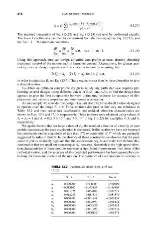
As an example we consider the design of a unit rise dwell-rise-dwell motion designed
to operate over the range F 2 ≥ 9. Three motions designed in this way are tabulated in
Table 13.2 and their associated acceleration and residual vibration characteristics are
shown in Figs. 13.9 and 13.10, respectively. These motions were obtained using values of
-7
-8
A 1 = A 2 = 1 and A 3 = 0.0, 5 ¥ 10 , and 7 ¥ 10 in Eq. (13.22) for examples 4, 5, and 6,
respectively.
We again observe that for large values of F 2, the residual vibration of a family of cam
profiles increases as the peak acceleration is decreased. In this section we have not imposed
the constraints on the magnitude of jerk (i.e., y≤¢) or continuity of y≤ which are generally
¯
¯
suggested by rules of thumb. In the absence of these constraints we observe that the peak
value of jerk is relatively high and that the acceleration begins and ends with definite dis-
continuities that are small but increasing as A 3 increases. Nonetheless the high-speed vibra-
tion characteristics of these motions represent a significant improvement over those of the
cycloidal motion, and the accuracy of this predicted performance has been assured by con-
trolling the harmonic content of the motion. The existence of such motions is contrary to

TABLE 13.2 Problem Solutions (Figs. 13.9 and
13.10)
No. 4 No. 5 No. 6
0.500000 0.500000 0.500000
a 0
-0.583802 -0.543883 -0.466909
a 1
0.095326 0.034106 -0.082227
a 3
-0.012015 0.011519 0.054570
a 5
0.000491 -0.001741 -0.005434
a 7
0.000000 -0.002399 -0.098142
b 2
0.000000 0.002835 0.078912
b 4
b 6 0.000000 -0.001293 -0.021730
0.000000 0.000152 0.001378
b 8