Page 102 - Carbonate Sedimentology and Sequence Stratigraphy

CHAPTER 6: FUNDAMENTALS OF SEQUENCE STRATIGRAPHY 93

global sea surface relative to a fixed datum on the planet, Distance (m)
such as the center of the Earth (Kendall and Lerche, 1988, 0 0 1165
p. 3). Estimating the eustatic sea level of past epochs is
very difficult as it depends on the use of proxy indicators
(Kendall and Lerche, 1988; Harrison, 1990).
Regression. The distinction betwen relative and eustatic sea
level is not sufficient to properly extract the sea-level sig- Depth (m)
nals from the stratigraphic record. Yet another distinction Dol. + Lst. Lst. + mar
needs to be made, the one between depositional and ero-
sional regression (Grabau, 1924 and Curray, 1964) or nor-
mal regression and forced regression (Posamentier et al.,
1992b). Depositional or normal regression develops where 450
the rate of sediment supply to the coastal zone exceeds the 0
rate of accommodation creation by relative sea-level rise.
Erosional or forced regression is caused by a fall of rela-
tive sea level; under this condition the shoreline shifts sea-
ward (and downward) irrespective of sediment supply. The
progradation of the highstand tract produces normal regres- TWT (ms)
sion, the downstepping from highstand to lowstand during
formation of the sequence boundary or the downward shift
within a falling-stage systems tract are examples of forced
regression.
Forced regression plays a pivotal role in the construction 25 Hz
of relative sea-level curves because it is clear evidence of 200
a relative sea-level fall, whereas the progradation and ret-
rogradation of highstand tracts and transgressive tracts may
be caused by changes of sea level or sediment supply (p.
94f; Jervey, 1988; Schlager, 1993). Distinguishing normal and
forced regression in siliciclastics relies on geometric criteria,
such as downstepping of the shelf break or incised valleys,
as well as facies patterns such as shoreface deposits with
erosional base (Posamentier et al., 1992b; Naish and Kamp,
1997). On carbonate platforms, downstepping of the margin
is a good criterion, particularly since the shelf break is often
better defined than in siliciclastics (chapter 3). Lithologic ev- 50 Hz
idence of exposure includes karst, soils, relicts of terrestrial
plants etc. Freshwater diagenesis alone is not diagnostic be-
cause it may also develop during depositional regression
when the system builds into the high supratidal zone, for
example on tidal flats (e.g. Halley and Harris, 1979; Gebelein
et al., 1980,p. 45).
Sea level from sequence anatomy. Stratigraphers are histo-
rians and, like most historians, are in danger of overinter-
preting the documents at hand. Sequence stratigraphy is
no exception. The literature contains numerous suggestions
on how certain features of sequence anatomy correlate with 100 Hz
the underlying sea-level curve and, conversely, how to con-
struct a sea-level curve from sequence anatomy. Most of
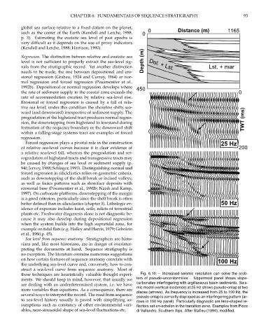
these techniques are heuristically valuable thought experi- Fig. 6.10.— Increased seismic resolution can solve the prob-
ments. We should keep in mind, however, that usually we lem of pseudo-unconformities . Uppermost panel shows slope-
carbonates interfingering with argillaceous basin sediments. Seis-
are dealing with an underdetermined system, i.e. we have
mic model (vertical incidence) at 25 Hz shows pseudo-onlap at two
more variables than equations. As a consequence, there are
places (arrows). As frequency is increased from 25 to 100 Hz, the
several ways to interpret the record. The road from sequence
pseudo-onlap is correctly displayed as an interfingering pattern (ar-
to sea-level history usually is paved with simplifying as- rows in 100 Hz panel). Particularly diagnostic are lens-shaped re-
sumptions such as constancy of other environmental vari- flectors set en-echelon in the transition zone. Examples from Picco
ables, near-sinusoidal shape of sea-level fluctuations etc. di Vallandro, Southern Alps. After Stafleu (1994), modified.