Page 256 - Chiral Separation Techniques

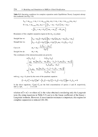
234 9 Modeling and Simulation in SMB for Chiral Purification

Table 9-3. Operating conditions for complete separation under Equilibrium Theory. Langmuir adsorp-
tion isotherms (see Fig. 9-8).
λ = m < m < ∞; m ( m m < m < m < m ( m m )
,
,
)
B 1,min 1 2,min 2 3 2 3 3,max 2 3
A {
F
,
0 < m < m 4,max ( m m ) = 1 λ + m + b C ( m − m )
A
A
4
2
3
2
3
3
2
A [
2
− λ + m + b C ( m – m ] − 4 λ m   
F
)
3
3
A
A
2
A
3
Boundaries of the complete separation region in the (m , m ) plane:
2 3
B [ F F G( ω )
ω
Straight line wr: λ − (1 + bC m + b C ω m = ω λ − G
G
B B )] 2
3
BB
B
G
λ λ − )
λ − λ 1 + bC m + b C A 3 A B λ A
Straight line wa: B [ A( F F λ m = (
B B )] 2
BB
( λ − m ) 2
Curve rb: m = m + B F 2
3
2
bC
BB
Straight line ab: m = m
3 2
The coordinates of the intersection points are given by:
(
(
a λ , ) ; b λ λ )
λ
,
B
A
B
A
G[
F(
 ω 2 ωω λω )( λ − λ ) + λ ω ( λω )] 
−
−
r   G , B G B A ω ) A G B F  
A (
 λ B λλ λ − F 
B
B
G[
λ λω )]
F(
 λω ωω λλ ) + ( − 
−
A
w   A G , B A ω ) A F 
A(
 λ B λλ − F 
B
with ω > ω > 0, given by the roots of the quadratic equation:
G F
)
1+ ( b C A F + bC ω 2 − λ 1+ ( bC B F ) + λ B 1+ ( b C A F )] ω + λ λ B = 0
F
A
A
A
B
B
B
[ A
F
In the above equations, C and C F are the feed concentrations of species A and B, respectively,
A B
and λ = Qb , (i = A, B)
i i
L
M
L
relation m = m + m where m is the value obtained considering only the Langmuir
j j j
term (by using equations in Table 9-3) and m is the linear coefficient of the linear +
Langmuir isotherm. However, if mass transfer resistance is important, this region for
complete separation is reduced [26–28].