Page 163 - Classification Parameter Estimation & State Estimation An Engg Approach Using MATLAB

152 SUPERVISED LEARNING

R
and h( ( , )) must be normalized to one, i.e. h( (z, z j ))dz ¼ 1 where
the integration extends over the entire measurement space.
The contribution of a single observation z j is h( (z, z j )). The contribu-
tions of all observations are summed to yield the final Parzen estimate:

1 X
^ p pðzj! k Þ¼ h ðz; z j Þ ð5:25Þ
N k
z j 2T k

The kernel h( ( , )) can be regarded as an interpolation function that
interpolates between the samples of the training set.
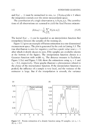
Figure 5.3 gives an example of Parzen estimation in a one-dimensional
measurement space. The plot is generated by the code in Listing 5.3. The
true distribution is zero for negative z and has a peak value near z ¼ 1
after which it slowly decays to zero. Fifty samples are available (shown
at the bottom of the figure). The interpolation function chosen is a
Gaussian function with width h . The distance measure is Euclidean.
Figure 5.3(a) and Figure 5.3(b) show the estimations using h ¼ 1 and
h ¼ 0:2, respectively. These graphs illustrate a phenomenon related to
the choice of the interpolation function. If the interpolation function is
peaked, the influence of a sample is very local, and the variance of the
estimator is large. But if the interpolation is smooth, the variance

(a) (b)

0.25
Parzen estimate 0.35 Parzen estimate
p(z|ω k ) p(z|ω k )
0.2 0.3
0.25
0.15
0.2
0.1 0.15
0.1
0.05
0.05
0 0
–2 0 2 4 6 8 10 –2 0 2 4 6 8 10
z z
Figure 5.3 Parzen estimation of a density function using 50 samples. (a) h ¼ 1.
(b) h ¼ 0:2