Page 165 - Classification Parameter Estimation & State Estimation An Engg Approach Using MATLAB

154 SUPERVISED LEARNING

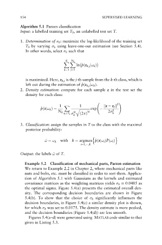
Algorithm 5.1 Parzen classification
Input: a labelled training set T S , an unlabelled test set T.

1. Determination of h : maximize the log-likelihood of the training set
T S by varying h using leave-one-out estimation (see Section 5.4).
In other words, select h such that

K N k
X X

p
ln ^ pðz k;j j! k Þ
k¼1 j¼1
is maximized. Here, z k,j is the j-th sample from the k-th class, which is
p
left out during the estimation of ^ p(z k,j j! k ).
2. Density estimation: compute for each sample z in the test set the
density for each class:

1 X 1 jjz z j jj 2 !
^ p pðzj! k Þ¼ ffiffiffiffiffiffiffiffiffiffiffiffiffi exp
q 2
N k N N 2
z j 2T k ð2 Þ h
h
3. Classification: assign the samples in T to the class with the maximal
posterior probability:

n o
^
P
p
^ ! ! ¼ ! k with k ¼ argmax ^ pðzj! i ÞPð! i Þ
i¼1; ;K
Output: the labels ^ ! of T.
!
Example 5.2 Classification of mechanical parts, Parzen estimation
We return to Example 2.2 in Chapter 2, where mechanical parts like
nuts and bolts, etc. must be classified in order to sort them. Applica-
tion of Algorithm 5.1 with Gaussians as the kernels and estimated
covariance matrices as the weighting matrices yields h ¼ 0:0485 as
the optimal sigma. Figure 5.4(a) presents the estimated overall den-
sity. The corresponding decision boundaries are shown in Figure
5.4(b). To show that the choice of h significantly influences the
decision boundaries, in Figure 5.4(c) a similar density plot is shown,
for which h was set to 0.0175. The density estimate is more peaked,
and the decision boundaries (Figure 5.4(d)) are less smooth.
Figures 5.4(a–d) were generated using MATLAB code similar to that
given in Listing 5.3.