Page 164 - Classification Parameter Estimation & State Estimation An Engg Approach Using MATLAB
P. 164
NONPARAMETRIC LEARNING                                       153

            decreases, but at the same time the estimate becomes a smoothed version
            of the true density. That is, the estimate becomes biased. By changing the
            width of the interpolation function one can balance between the bias and
            the variance. Of course, both types of errors can be reduced by enlarge-
            ment of the training set.


            Listing 5.3
            The following PRTools listing generates plots similar to those in Figure
            5.3. It generates 50 samples from a  (a, b) distribution with a ¼ 2 and
            b ¼ 1:5, and then estimates the density using the Parzen method with
            two different kernel widths.

            n ¼ 50; a ¼ 2; b ¼ 1.5;
            x ¼ ( 2:0.01:10)’; y ¼ gampdf(x,a,b);      % Generate function
            z ¼ dataset(gamrnd(a,b,n,1),genlab(n));    % Generate dataset
            w ¼ parzenm(z,1);                          % Parzen, sigma ¼ 1
            figure; scatterd(z); axis([ 2 10 0 0.3]);
            plotm(w,1); hold on; plot(x,y,’:’);
            w ¼ parzenm(z,0.2);                        % Parzen, sigma ¼ 0.2
            figure; scatterd(z); axis([ 2 10 0 0.3]);
            plotm(w,1); hold on; plot(x,y,’:’);

            In the N-dimensional case, various interpolation functions are useful.
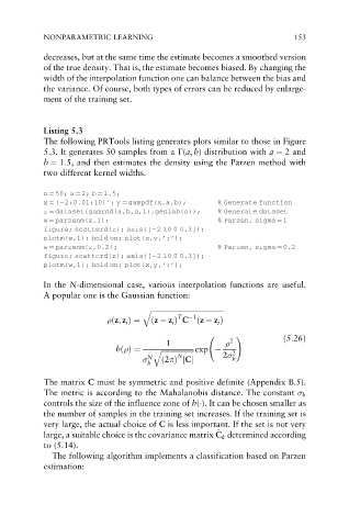
            A popular one is the Gaussian function:

                                    q ffiffiffiffiffiffiffiffiffiffiffiffiffiffiffiffiffiffiffiffiffiffiffiffiffiffiffiffiffiffiffiffiffiffiffiffiffiffiffiffiffi
                                             T   1
                            ðz; z j Þ¼  ðz   z j Þ C ðz   z j Þ
                                                           !           ð5:26Þ
                                          1                2
                              hð Þ¼    q ffiffiffiffiffiffiffiffiffiffiffiffiffiffiffiffiffiffiffi exp    2  2
                                             N
                                      N  ð2 Þ jCj         h
                                     h
            The matrix C must be symmetric and positive definite (Appendix B.5).
            The metric is according to the Mahalanobis distance. The constant   h
            controls the size of the influence zone of h( ). It can be chosen smaller as
            the number of samples in the training set increases. If the training set is
            very large, the actual choice of C is less important. If the set is not very
                                                      ^
                                                      C
            large, a suitable choice is the covariance matrix C k determined according
            to (5.14).
              The following algorithm implements a classification based on Parzen
            estimation:

