Page 120 - Classification Parameter Estimation & State Estimation An Engg Approach Using MATLAB
P. 120
CONTINUOUS STATE VARIABLES                                   109

              A better approach is the so-called iterated extended Kalman filter
            (IEKF). Here, the approximation is made that both the predicted state
            and the measurement noise are normally distributed. With that, the
            posterior probability density (4.9)


                                      1
                         pðxðiÞjZðiÞÞ ¼ pðxðiÞjZði   1ÞÞpðzðiÞjxðiÞÞ   ð4:50Þ
                                      c

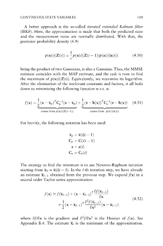
            being the product of two Gaussians, is also a Gaussian. Thus, the MMSE
            estimate coincides with the MAP estimate, and the task is now to find
            the maximum of p(x(i)jZ(i)). Equivalently, we maximize its logarithm.
            After the elimination of the irrelevant constants and factors, it all boils
            down to minimizing the following function w.r.t. x:

                     1        T   1         1          T   1
              fðxÞ¼ ðx   x p Þ C ðx   x p Þ þ ðz   hðxÞÞ C ðz   hðxÞÞ  ð4:51Þ
                                p
                                                         v
                     2                      2
                     |fflfflfflfflfflfflfflfflfflfflfflfflfflfflfflfflfflfflfflffl{zfflfflfflfflfflfflfflfflfflfflfflfflfflfflfflfflfflfflfflffl}  |fflfflfflfflfflfflfflfflfflfflfflfflfflfflfflfflfflfflfflfflfflfflfflffl{zfflfflfflfflfflfflfflfflfflfflfflfflfflfflfflfflfflfflfflfflfflfflfflffl}
                       comes from pðxðiÞjZði 1ÞÞ  comes from pðzðiÞjxðiÞÞ
            For brevity, the following notation has been used:


                                      x p ¼ xðiji   1Þ
                                     C p ¼ Cðiji   1Þ
                                       z ¼ zðiÞ
                                     C v ¼ C v ðiÞ


            The strategy to find the minimum is to use Newton–Raphson iteration
            starting from x 0 ¼ x(iji   1). In the ‘-th iteration step, we have already
            an estimate x ‘ 1 obtained from the previous step. We expand f(x)in a
            second order Taylor series approximation:


                                                 T  qfðx ‘ 1 Þ
                         fðxÞffi fðx ‘ 1 Þþ ðx   x ‘ 1 Þ
                                                     qx
                                                                       ð4:52Þ
                                               2
                                  1         T  q fðx ‘ 1 Þ
                                þ ðx   x ‘ 1 Þ         ðx   x ‘ 1 Þ
                                  2             qx 2
                                            2
                                                 2
            where qf/qx is the gradient and q f/qx is the Hessian of f(x). See
            Appendix B.4. The estimate x ‘ is the minimum of the approximation.

