Page 121 - Classification Parameter Estimation & State Estimation An Engg Approach Using MATLAB

110 STATE ESTIMATION

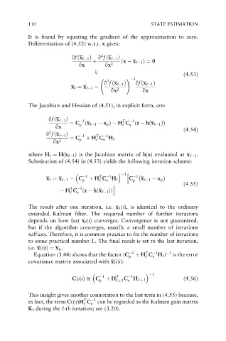
It is found by equating the gradient of the approximation to zero.
Differentiation of (4.52) w.r.t. x gives:

2
qfðx ‘ 1 Þ q fðx ‘ 1 Þ
þ ðx x ‘ 1 Þ¼ 0
qx qx 2
+
ð4:53Þ
! 1
2
q fðx ‘ 1 Þ qfðx ‘ 1 Þ
x ‘ ¼ x ‘ 1
qx 2 qx
The Jacobian and Hessian of (4.51), in explicit form, are:

qfðx ‘ 1 Þ 1 T 1
¼ C ðx ‘ 1 x p Þ H C ðz hðx ‘ 1 ÞÞ
qx p ‘ v
ð4:54Þ
2
q fðx ‘ 1 Þ 1 T 1
¼ C þ H C H ‘
qx 2 p ‘ v
where H ‘ ¼ H(x ‘ 1 ) is the Jacobian matrix of h(x) evaluated at x ‘ 1 .
Substitution of (4.54) in (4.53) yields the following iteration scheme:

1
h
1
T
x ‘ ¼ x ‘ 1 C 1 þ H C H ‘ C 1 x ‘ 1 x p
p ‘ v p
ð4:55Þ
i
T 1
H C ðz hðx ‘ 1 ÞÞ
‘ v
The result after one iteration, i.e. x 1 (i), is identical to the ordinary
extended Kalman filter. The required number of further iterations
depends on how fast x ‘ (i) converges. Convergence is not guaranteed,
but if the algorithm converges, usually a small number of iterations
suffices. Therefore, it is common practice to fix the number of iterations
to some practical number L. The final result is set to the last iteration,
i.e. x(iji) ¼ x L .
1
T
Equation (3.44) shows that the factor (C 1 þ H C H ‘ ) 1 is the error
p ‘ v
covariance matrix associated with x(iji):
1

1
CðijiÞffi C 1 þ H T C H Lþ1 ð4:56Þ
v
Lþ1
p
This insight gives another connotation to the last term in (4.55) because,
T
in fact, the term C(iji)H C 1 can be regarded as the Kalman gain matrix
v
‘
K ‘ during the ‘-th iteration; see (3.20).