
Page 126 - Classification Parameter Estimation & State Estimation An Engg Approach Using MATLAB
P. 126
DISCRETE STATE VARIABLES 115
P (1|1) P (2 | 2) P (3 | 3) P (4 | 4)
t
t
t
t
P (2 |1) P (3| 2)
t
t
Pt (4 | 3)
ω ω ω ω
1 2 3 4
P (3|1) P (4 | 2)
t
t
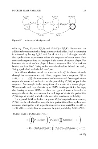
Figure 4.13 A four-state left–right model
with ! K . Thus, P 0 (k) ¼ d(k,1) and P t (kjK) ¼ d(k,K). Sometimes, an
additional constraint is that large jumps are forbidden. Such a constraint
is enforced by letting P t (kj‘) ¼ 0 for all k >‘ þ . Left–right models
find applications in processes where the sequence of states must obey
some ordering over time. An example is the stroke of a tennis player. For
instance, the service of the player follows a sequence like: ‘take position
behind the base line’, ‘bring racket over the shoulder behind the back’,
‘bring up the ball with the left arm’, etc.
In a hidden Markov model the state variable x(i) is observable only
through its measurements z(i). Now, suppose that a sequence Z(i) ¼
fz(0), z(1), .. . , z(i)g of measurements has been observed. Some applications
require the numerical evaluation of the probability P(Z(i)) of particular
sequence. An example is the recognition of a stroke of a tennis player.
We can model each type of stroke by an HMM that is specific for that type,
thus having as many HMMs as there are types of strokes. In order to
recognize the stroke, we calculate for each type of stroke the probability
P(Z(i)jtype of stroke) and select the one with maximum probability.
For a given HMM, and a fixed sequence Z(i) of acquired measurements,
P(Z(i)) can be calculated by using the joint probability of having the meas-
urements Z(i) together with a specific sequence of state variables, i.e. X(i) ¼
fx(0), x(1), ... , x(i)g. First we calculate the joint probability P(X(i), Z(i)):
PðXðiÞ; ZðiÞÞ ¼ PðZðiÞjXðiÞÞPðXðiÞÞ
i ! i !
Y Y
¼ P z ðzðjÞjxðjÞÞ P 0 ðxð0ÞÞ P t ðxðjÞjxðj 1ÞÞ
j¼0 j¼1
i
Y
¼ P 0 ðxð0ÞÞP z ðzð0Þjxð0ÞÞ ðP z ðzðjÞjxðjÞÞP t ðxðjÞjxðj 1ÞÞÞ
j¼1
ð4:57Þ