
Page 128 - Classification Parameter Estimation & State Estimation An Engg Approach Using MATLAB
P. 128
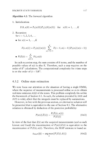
DISCRETE STATE VARIABLES                                     117

            Algorithm 4.1: The forward algorithm

            1. Initialization:

                                       ð
                   Fð0; xð0Þ¼ P 0 xð0Þð  ÞP z zð0Þjxð0ÞÞ  for  xð0Þ¼ 1; ... ; K
            2. Recursion:
               for i ¼ 1, 2, 3, 4, ...
               . for x(i) ¼ 1, .. . , K

                                            K
                                           X
                     ð
                    Fi;xðiÞÞ ¼ P z zðiÞjxðiÞð  Þ  Fði   1;xði   1ÞÞP t ðxðiÞjxði   1ÞÞ
                                         xði 1Þ¼1
                           K
                           P
               . P(Z(i)) ¼    F(i, x(i))
                          x(i)¼1
              In each recursion step, the sum consists of K terms, and the number of
            possible values of x(i) is also K. Therefore, such a step requires on the
                     2
            order of K calculations. The computational complexity for i time steps
                                   2
            is on the order of (i þ 1)K .


            4.3.2  Online state estimation

            We now focus our attention on the situation of having a single HMM,
            where the sequence of measurements is processed online so as to obtain
                             x
            real-time estimates ^ x(iji) of the states. This problem completely fits within
            the framework of Section 4.1. As such, the solution provided by (4.8) and
            (4.9) is valid, albeit that the integrals must be replaced by summations.
              However, in line with the previous section, an alternative solution will
            be presented that is equivalent to the one of Section 4.1. The alternative
            solution is obtained by deduction of the posterior probability:

                                             PðZðiÞ; xðiÞÞ
                                PðxðiÞjZðiÞÞ ¼                         ð4:61Þ
                                               PðZðiÞÞ
            In view of the fact that Z(i) are the acquired measurements (and as such
            known and fixed) the maximization of P(x(i)jZ(i)) is equivalent to the
            maximization of P(Z(i), x(i)). Therefore, the MAP estimate is found as:

                             ^ x x MAP ðijiÞ¼ arg maxfPðZðiÞ; kÞÞg     ð4:62Þ
                                           k