Page 115 - Classification Parameter Estimation & State Estimation An Engg Approach Using MATLAB

104 STATE ESTIMATION

with the Jacobian matrix:

1 0
HðxÞ¼ ð4:41Þ
0 U expð DÞ
The best fitted parameters of this model are as follows:

Volume control Substance flow Output flow Measurement system

¼ 1 (s) f ¼ 0:1 (lit/s) V ref ¼ 4000 (lit) v 1 ¼ 16 (lit)
2
V 0 ¼ 4001 (lit) w 2 ¼ 0:9 (lit/s) c ¼ 1 (lit/s) U ¼ 1000 (V)
¼ 0:95 (1/s) ¼ 100
¼ 0:1225 (lit/s) ¼ 0:02 (V)
w 1 v 2
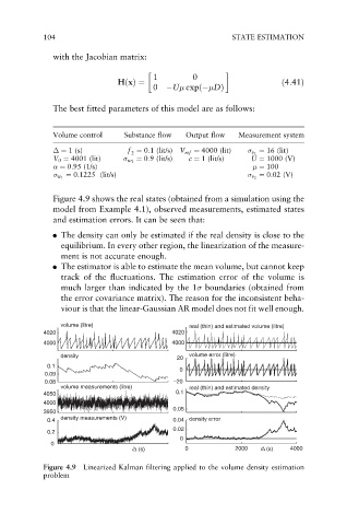
Figure 4.9 shows the real states (obtained from a simulation using the
model from Example 4.1), observed measurements, estimated states
and estimation errors. It can be seen that:

. The density can only be estimated if the real density is close to the
equilibrium. In every other region, the linearization of the measure-
ment is not accurate enough.
. The estimator is able to estimate the mean volume, but cannot keep
track of the fluctuations. The estimation error of the volume is
much larger than indicated by the 1 boundaries (obtained from
the error covariance matrix). The reason for the inconsistent beha-
viour is that the linear-Gaussian AR model does not fit well enough.

volume (litre) real (thin) and estimated volume (litre)
4020 4020
4000 4000
density 20 volume error (litre)
0.1
0
0.09
0.08 –20
volume measurements (litre) real (thin) and estimated density
4050 0.1
4000
0.05
3950
density measurements (V)
0.4 0.04 density error
0.02
0.2
0
0
i∆ (s) 0 2000 i∆ (s) 4000
Figure 4.9 Linearized Kalman filtering applied to the volume density estimation
problem