Page 114 - Classification Parameter Estimation & State Estimation An Engg Approach Using MATLAB

CONTINUOUS STATE VARIABLES 103

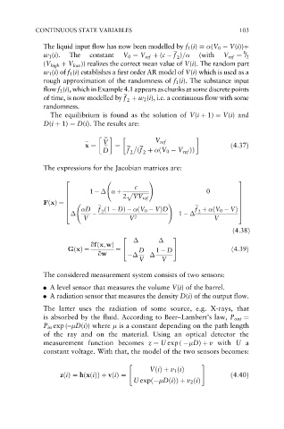
The liquid input flow has now been modelled by f 1 (i) ¼ (V 0 V(i))þ
w 1 (i). The constant V 0 ¼ V ref þ (c f )= (with 1
2 V ref ¼ / 2
(V high þ V low )) realizes the correct mean value of V(i). The random part
w 1 (i)of f 1 (i) establishes a first order AR model of V(i) which is used as a
rough approximation of the randomness of f 1 (i). The substance input
flow f 2 (i), which in Example 4.1 appears as chunks at some discrete points
of time, is now modelled by f þ w 2 (i), i.e. a continuous flow with some
2
randomness.
The equilibrium is found as the solution of V(i þ 1) ¼ V(i) and
D(i þ 1) ¼ D(i). The results are:

¼
¼ V V ref
x ¼ ¼ ¼ ð4:37Þ
D f 2 ðf þ ðV 0 V ref ÞÞ
2
The expressions for the Jacobian matrices are:

2 3
!
c
0
6 1 þ p ffiffiffiffiffiffiffiffiffiffiffiffi 7
2
6 VV ref 7
6 7
!
FðxÞ¼ 6
7
6 D f ð1 DÞ ðV 0 VÞD f þ ðV 0 VÞ 7
1
4 2 2 5
V V 2 V
ð4:38Þ

2 3
qfðx;wÞ
GðxÞ¼ ¼ 4 D 1 D 5 ð4:39Þ
qw
V V
The considered measurement system consists of two sensors:
. A level sensor that measures the volume V(i) of the barrel.
. A radiation sensor that measures the density D(i) of the output flow.
The latter uses the radiation of some source, e.g. X-rays, that
is absorbed by the fluid. According to Beer–Lambert’s law, P out ¼
P in exp ( D(i)) where is a constant depending on the path length
of the ray and on the material. Using an optical detector the
measurement function becomes z ¼ U exp ( D) þ v with U a
constant voltage. With that, the model of the two sensors becomes:

" #
VðiÞþ v 1 ðiÞ
ð
zðiÞ¼ hxðiÞÞ þ vðiÞ¼ ð4:40Þ
ð
U exp DðiÞÞ þ v 2 ðiÞ