Page 113 - Classification Parameter Estimation & State Estimation An Engg Approach Using MATLAB

102 STATE ESTIMATION

¼ ¼
By interpreting the term (I F(x))x as a constant control input, and
¼ ¼ ¼
by compensating the offset term h(x) H(x)x in the measurement
vector, these equations become equivalent to (4.11) and (4.25). This
allows the direct application of the DKF as given in (4.28) and (4.27).
Many practical implementations of the discrete Kalman filter are
inherently linearized Kalman filters because physical processes are sel-
dom exactly linear, and often a linear model is only an approximation of
the real process.

Example 4.4 The swinging pendulum
The swinging pendulum from Example 4.2 is described by (4.23):

€
_

maðtÞ cos ðtÞþ mR ðtÞ¼ mg sin ðtÞ mk ðtÞ
R
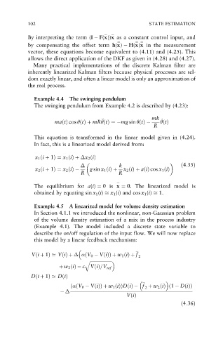
This equation is transformed in the linear model given in (4.24).
In fact, this is a linearized model derived from:

x 1 ði þ 1Þ¼ x 1 ðiÞþ x 2 ðiÞ
k ð4:35Þ
x 2 ði þ 1Þ¼ x 2 ðiÞ g sin x 1 ðiÞþ x 2 ðiÞþ aðiÞ cos x 1 ðiÞ
R R

¼
The equilibrium for a(i) ¼ 0is x ¼ 0. The linearized model is
obtained by equating sin x 1 (i) ffi x 1 (i) and cos x 1 (i) ffi 1.

Example 4.5 A linearized model for volume density estimation
In Section 4.1.1 we introduced the nonlinear, non-Gaussian problem
of the volume density estimation of a mix in the process industry
(Example 4.1). The model included a discrete state variable to
describe the on/off regulation of the input flow. We will now replace
this model by a linear feedback mechanism:

Vði þ 1Þ’ VðiÞþ ðV 0 VðiÞÞ þ w 1 ðiÞþ f 2
q ffiffiffiffiffiffiffiffiffiffiffiffiffiffiffiffiffiffiffiffi
þw 2 ðiÞ c VðiÞ=V ref
Dði þ 1Þ’ DðiÞ

ð ðV 0 VðiÞÞ þ w 1 ðiÞÞDðiÞ f þ w 2 ðiÞ 1 DðiÞÞ
ð
2

VðiÞ
ð4:36Þ