Page 110 - Classification Parameter Estimation & State Estimation An Engg Approach Using MATLAB

CONTINUOUS STATE VARIABLES 99

Example 4.3 Application to the swinging pendulum
In this example we reconsider the mechanical system shown in
Figure 4.6, and described in Example 4.2. Suppose a gyroscope meas-
_
ures the angular speed (t) at regular intervals of 0:4 s. The discrete

model in Example 4.2 uses a sampling period of ¼ 0:01 s. We could
increase the sampling period to 0:4 s in order to match it with the
sampling period of the measurements, but then the applied discrete
approximation would be poor. Instead, we model the measurements
with a time variant model: z(i) ¼ H(i)x(i) þ v(i) where both H(i) and
C v (i) are always zero except for those i that are multiples of 40:

½01Š if modði; 40Þ¼ 0
HðiÞ¼ ð4:30Þ
0 elsewhere
The effect of such a measurement matrix is that during 39 consecutive
cycles of the loop only predictions take place. During these cycles
H(i) ¼ 0, and consequently the Kalman gains are zero. The corres-
ponding updates would have no effect, and can be skipped. Only
during each 40th cycle H(i) 6¼ 0, and a useful update takes place.
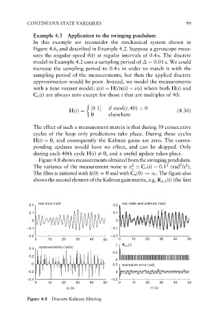
Figure4.8showsmeasurementsobtainedfromtheswingingpendulum.
2
2
2
2
The variance of the measurement noise is C v (i) ¼ 0:1 (rad /s ).
v
The filter is initiated with x(0) ¼ 0 and with C x (0) !1. The figure also
shows the second element of the Kalman gain matrix, e.g. K 2,1 (i) (the first

real state (rad) real state and estimate (rad)
0.2 0.2
0.1 0.1
0 0
– 0.1 – 0.1
– 0.2 – 0.2
0 10 20 30 40 50 0 10 20 30 40 50
1 K 2,1 (i)
measurements (rad/s)
0.4
0.5
0.2
0
0 0.2 estimation error (rad)
– 0.2 0
– 0.4 – 0.2
0 10 20 30 40 50 0 10 20 30 40 50
i∆ (s) i∆ (s)
Figure 4.8 Discrete Kalman filtering