Page 105 - Classification Parameter Estimation & State Estimation An Engg Approach Using MATLAB

94 STATE ESTIMATION

The equations are valid if the system is in the steady state, i.e.
2
2
when (i) ¼ (i þ 1) and E[x(i þ 1)x(i)] ¼ E[x(i)x(i 1)]. For this
x x
2
2
situation the abbreviated notation (1) is used. Furthermore,
x x
r k denotes the autocorrelation between x(i) and x(i þ k). That is,
2
E[x(i)x(i þ k)] ¼ Cov[x(i)x(i þ k)] ¼ r k (only valid in the steady state).
x
See also Section 8.1.5 and Appendix C.2.
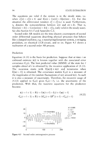
Second order AR models are the time-discrete counterparts of second
order differential equations describing physical processes that behave
like a damped oscillator, e.g. a mass/spring/dampener system, a swinging
pendulum, an electrical LCR-circuit, and so on. Figure 4.5 shows a
realization of a second order AR process.
Prediction

Equation (4.13) is the basis for prediction. Suppose that at time i an
x
unbiased estimate ^ x(i) is known together with the associated error
covariance C e (i). The best predicted value (MMSE) of the state for ‘
samples ahead of i is obtained by the recursive application of (4.13).
The recursion starts with E[x(i)] ¼ ^ x(i) and terminates when
x
E[x(i þ ‘)] is obtained. The covariance matrix C e (i)is a measure of
x
the magnitudes of the random fluctuations of x(i)around ^ x(i). As such
it is also a measure of uncertainty. Therefore, the recursive usage of
(4.13) applied to C e (i)gives C e (i þ ‘), i.e. the uncertainty of the
prediction. With that, the recursive equations for the prediction
become:

x
^ x xði þ ‘ þ 1Þ¼ Fði þ ‘Þ^ xði þ ‘Þþ Lði þ ‘Þuði þ ‘Þ
ð4:22Þ
T
C e ði þ ‘ þ 1Þ¼ Fði þ ‘ÞC e ði þ ‘ÞF ði þ ‘Þþ C w ði þ ‘Þ

d = 0.995
20
f = 0.1
+1σ boundary α = 1.61
10 β = – 0.99
σ = 1
2
w
0 2 (∞) = 145.8
σ
x
–10
–1σ boundary
–20
0 100 i 200
Figure 4.5 Second order autoregressive process