Page 107 - Classification Parameter Estimation & State Estimation An Engg Approach Using MATLAB

96 STATE ESTIMATION

(a) (b)
0.2 real state and prediction (rad) 100% σ pred /σ x
0.1
lead • ∆ = 2 (s)
0 50% ↓
–0.1
–0.2 0%
0 10 20 30 40 50 0 1 2 3 4 5
i∆ (s) lead • ∆ (s)
0.2 prediction error (rad) 0.2 real state and prediction (rad)
0.1 0.1
0 0
–0.1 –0.1
–0.2 –0.2
–10 0 10 20 30 40 0 10 20 30 40 50
lead • ∆ (s) i∆ (s)
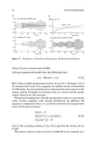
Figure 4.7 Prediction. (a) Fixed interval prediction. (b) Fixed lead prediction

Linear-Gaussian measurement models
A linear measurement model takes the following form:

zðiÞ¼ HðiÞxðiÞþ vðiÞ ð4:25Þ

H(i) is the so-called measurement matrix.Itisan N M matrix. v(i)is
the measurement noise. It is a sequence of random vectors of dimension
N. Obviously, the measurement noise represents the noise sources in the
sensory system. Examples are thermal noise in a sensor and the quant-
ization errors of an AD converter.
The general assumption is that the measurement noise is a zero mean,
white random sequence with normal distribution. In addition, the
sequence is supposed to have no correlation between the measurement
noise and the process noise:

E½vðiފ ¼ 0
T

E vðiÞv ð jÞ ¼ C v ðiÞdði; jÞ ð4:26Þ
T

E vðiÞw ð jÞ ¼ 0

C v (i) is the covariance matrix of v(i). C v (i) specifies the density of v(i)
in full.
The sensory system is time invariant if neither H nor C v depends on i.