
Page 172 - Classification Parameter Estimation & State Estimation An Engg Approach Using MATLAB
P. 172
NONPARAMETRIC LEARNING 161
2. Condensing: use 1-NNR classification with the current T STORE to
classify a sample in T GRABBAG ; if classified correctly, the sample is
retained in T GRABBAG , otherwise it is moved from T GRABBAG to
T STORE ; repeat this operation for all other samples in T GRABBAG .
3. Termination: if one complete pass is made through step 2 with no
transfer from T GRABBAG to T STORE ,orif T GRABBAG is empty, then
terminate; else go to step 2.
Output: a subset of T S .
The effect of this algorithm is that in regions where the training set is
overcrowded with samples of the same class most of these samples will
be removed. The remaining set will, hopefully, contain samples close to
the Bayes decision boundaries.
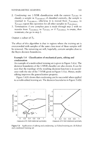
Example 5.4 Classification of mechanical parts, editing and
condensation
An example of a multi-edited training set is given in Figure 5.6(a). The
decision boundaries of the 1-NNR classifier are also shown. It can be
seen that the topology of the resulting decision function is in accord-
ance with the one of the 7-NNR given in Figure 5.5(a). Hence, multi-
editing improves the generalization property.
Figure 5.6(b) shows that condensing can be successful when applied
to a multi-edited training set. The decision boundaries in Figure 5.6(b)
1 0.8 1
measure of eccentricity 0.6 measure of eccentricity 0.6
0.8
0.4
0.4
0.2
0 0.2 0
0 0.2 0.4 0.6 0.8 1 0 0.2 0.4 0.6 0.8 1
measure of 6–fold rotational symmetry measure of 6–fold rotational symmetry
Figure 5.6 Application of editing and condensing. (a) Edited training set. (b) Edited
and condensed training set