Page 169 - Classification Parameter Estimation & State Estimation An Engg Approach Using MATLAB

158 SUPERVISED LEARNING

(a) (b)
1
1 0.8
measure of eccentricity 0.6 measure of eccentricity 0.6
0.8

0.4
0.4
0.2
0
0 0.2
0 0.2 0.4 0.6 0.8 1 0 0.2 0.4 0.6 0.8 1
measure of six-fold rotational symmetry measure of six-fold rotational symmetry
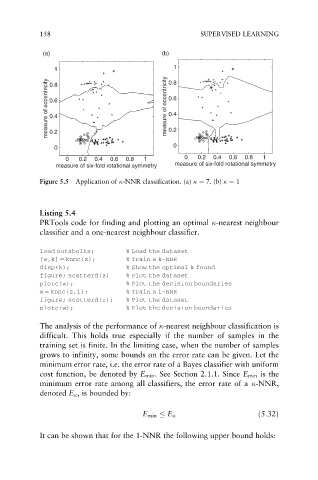
Figure 5.5 Application of -NNR classification. (a) ¼ 7. (b) ¼ 1

Listing 5.4
PRTools code for finding and plotting an optimal -nearest neighbour
classifier and a one-nearest neighbour classifier.

load nutsbolts; % Load the dataset
[w,k] ¼ knnc(z); % Train a k-NNR
disp(k); % Show the optimal k found
figure; scatterd(z) % Plot the dataset
plotc(w); % Plot the decision boundaries
w ¼ knnc(z,1); % Train a 1-NNR
figure; scatterd(z); % Plot the dataset
plotc(w); % Plot the decision boundaries
The analysis of the performance of -nearest neighbour classification is
difficult. This holds true especially if the number of samples in the
training set is finite. In the limiting case, when the number of samples
grows to infinity, some bounds on the error rate can be given. Let the
minimum error rate, i.e. the error rate of a Bayes classifier with uniform
cost function, be denoted by E min . See Section 2.1.1. Since E min is the
minimum error rate among all classifiers, the error rate of a -NNR,
denoted E , is bounded by:

E min E ð5:32Þ

It can be shown that for the 1-NNR the following upper bound holds: