Page 259 - Classification Parameter Estimation & State Estimation An Engg Approach Using MATLAB

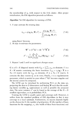
248 UNSUPERVISED LEARNING

the membership of z n with respect to the k-th cluster. After proper
initialization, the EM algorithm proceeds as follows:

Algorithm 7.6: EM algorithm for training a GTM:

1. E step: estimate the missing data:

^
2
W

^
k
2

W
x x n;k ¼ pðq jz n ; W; ^ Þ¼ pðz n jq ; W; ^ Þ ð7:41Þ
k K
W

P ^ 2
pðz n jq ; W; ^ Þ
k
k¼1
using Bayes’ theorem.
2. M step: re-estimate the parameters:
T
^ T
T
1 T
W ¼ð G þ IÞ X Z ð7:42Þ
W
1 N S K
2 X X ^ 2
W
^ ¼ x x n;k kWg ðq Þ z n k ð7:43Þ
k
N S N
n¼1 k¼1
3. Repeat 1 and 2 until no significant changes occur.
z
N S
P
G is a K K diagonal matrix with G kk ¼ n¼1 n,k as elements. is a
K M matrix containing the basis functions: k,m ¼
m (q ). X is a
k
N S K matrix with the x n,k as elements. Z is a N S N matrix. It
x
T
contains the data vectors z as its rows. Finally, is a regularization
n
T
parameter, which is needed in cases where G becomes singular and
the inverse cannot be computed.
The GTM can be initialized by performing PCA on the data set,
projecting the data to D dimensions and finding W such that the result-
ing latent variables q approximate as well as possible the projected
n
2
data. The noise variance can be found as the average of the N D
smallest eigenvalues, as in probabilistic PCA.
Training the GTM is usually quick and converges well. However, it
suffers from the standard problem of EM algorithms in that it may
converge to a local optimum. Furthermore, its success depends highly
on the choices for K (the number of grid points), M (the number of basis
functions for the mapping), ’ (the width of these basis functions) and