Page 163 - Compact Numerical Methods For Computers

152 Compact numerical methods for computers
generated without risking, at the very least, unnecessary function evaluations
which, after all, one is trying to avoid by using more of the information about the
function S(b) than the rather conservative direct search methods above.
At this juncture we can consider combining the success-failure algorithm with
inverse interpolation. One choice, made in algorithm 22, is to take the initial
point in the success-failure procedure as b Then ‘successes’ lower the function
0
value. Ultimately, however, a ‘failure’ will follow a ‘success unless u=b 0 is
minimal, even if the procedure begins with a string of ‘failures’. Call the position
at the last ‘failure’ b , and the position at the ‘success’ which preceded it b . (Note
2
1
that b 1 has to be the lowest point found so far.) Then S(b ) is less than either
1
S(b ) or S(b ) and the three points define a V-shape which ensures that the
0
2
interpolating parabola (13.5) will not be used to extrapolate.
Alternatively, as in algorithm 17 below, any of the following combinations of
events lead to a V-shaped triple of points with b 1 the lowest of the three:
(i) initial point, success, failure (b , b , b )
0
2
1
(ii) success, success, failure (b , b , b )
0
2
1
(iii) initial point, failure, failure (b , b , b ).
1
2
0
Consider then the three points defined by b , b , b where b, occupies the middle
0
1
2
position and where, using the notation
S =S(b ) (13.7)
j
j
for brevity,
S <S 0 (13.8)
1
and
S <S . (13.9)
1 2
Excluding the exceptional cases that the function is flat or otherwise perverse, so
that at least one of the conditions (13.8) or (13.9) is an inequality, the interpola-
ting parabola will have its minimum between b and b . Note now that we can
0 2
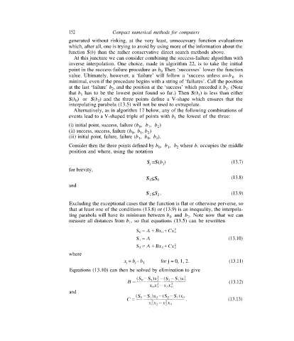
measure all distances from b , so that equations (13.5) can be rewritten
1
(13.10)
where
x = b - b 1 for j = 0, 1, 2. (13.11)
j
j
Equations (13.10) can then be solved by elimination to give
(13.12)
and
(13.13)