
Page 167 - Compact Numerical Methods For Computers
P. 167
156 Compact numerical methods for computers
Algorithm 17. Minimisation of a function of one variable (cont.)
begin {evaluate function if argument has been changed}
fii := fn1d(xii,notcomp); ifn := ifn+1;
if notcomp then fii := big;
if fii<s1 then
begin
s1 := fii; x1 := xii; {save new & better function, argument}
writeln(‘New min f(‘,x1,‘)=‘,s1);
end;
end; {evaluate function for parabolic inverse interpolation}
end; {if not zerodivide situation}
writeln(ifn,’ evalnsf(‘,x1,‘)=‘,s1);
s0 := s1; {to save function value in case of new iteration}
until (bb=x1); {Iterate until minimum does not change. We could
use reltest in this termination condition,}
writeln(‘Apparent minimum is f(‘,bb,‘)=‘,s1);
writeln(‘after ‘jfn,’ function evaluations’);
fnminval := s1; {store value for return to calling program}
end; {alg17.pas == min1d}
The driver program DR1617.PAS on the software diskette allows grid search to be used to
localise a minimum, with its precise locution found using the one-dimensional minimiser above.
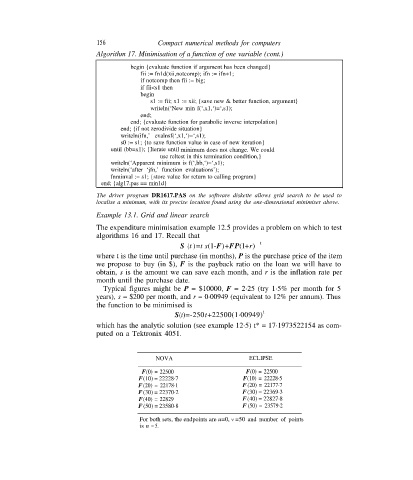
Example 13.1. Grid and linear search
The expenditure minimisation example 12.5 provides a problem on which to test
algorithms 16 and 17. Recall that
t
S (t )=t s(l-F)+FP(l+r)
where t is the time until purchase (in months), P is the purchase price of the item
we propose to buy (in $), F is the payback ratio on the loan we will have to
obtain, s is the amount we can save each month, and r is the inflation rate per
month until the purchase date.
Typical figures might be P = $10000, F = 2·25 (try 1·5% per month for 5
years), s = $200 per month, and r = 0·00949 (equivalent to 12% per annum). Thus
the function to be minimised is
t
S(t)=-250t+22500(1·00949)
which has the analytic solution (see example 12·5) t* = 17·1973522154 as com-
puted on a Tektronix 4051.
NOVA ECLIPSE
F(0) = 22500 F(0) = 22500
F(10) = 22228·7 F(10) = 22228·5
F(20) = 22178·1 F(20) = 22177·7
F(30) = 22370·2 F(30) = 22369·3
F(40) = 22829 F(40) = 22827·8
F(50) = 23580·8 F (50) = 23579·2
For both sets, the endpoints are u=0, v =50 and number of points
is n = 5.