Page 164 - Compact Numerical Methods For Computers

One-dimensional problems 153
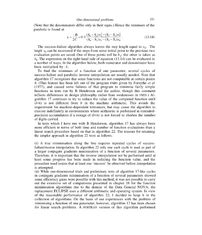
(Note that the denominators differ only in their signs.) Hence the minimum of the
parabola is found at

(13.14)

The success-failure algorithm always leaves the step length equal to x . The
2
length x can be recovered if the steps from some initial point to the previous two
0
evaluation points are saved. One of these points will be b ; the other is taken as
1
b . The expression on the right-hand side of equation (13.14) can be evaluated in
0
a number of ways. In the algorithm below, both numerator and denominator have
been multiplied by -1.
To find the minimum of a function of one parameter, several cycles of
success-failure and parabolic inverse interpolation are usually needed. Note that
algorithm 17 recognises that some functions are not computable at certain points
b. (This feature has been left out of the program FMIN given by Forsythe et al
(1977), and caused some failures of that program to minimise fairly simple
functions in tests run by B Henderson and the author, though this comment
reflects differences in design philosophy rather than weaknesses in FMIN.) Al-
gorithm 17 continues to try to reduce the value of the computed function until
(b+h) is not different from b in the machine arithmetic. This avoids the
requirement for machine-dependent tolerances, but may cause the algorithm to
execute indefinitely in environments where arithmetic is performed in extended-
precision accumulators if a storage of (b+h) is not forced to shorten the number
of digits carried.
In tests which I have run with B Henderson, algorithm 17 has always been
more efficient in terms of both time and number of function evaluations than a
linear search procedure based on that in algorithm 22. The reasons for retaining
the simpler approach in algorithm 22 were as follows.
(i) A true minimisation along the line requires repeated cycles of success-
failure/inverse interpolation. In algorithm 22 only one such cycle is used as part of
a larger conjugate gradients minimisation of a function of several parameters.
Therefore, it is important that the inverse interpolation not be performed until at
least some progress has been made in reducing the function value, and the
procedure used insists that at least one ‘success’ be observed before interpolation
is attempted.
(ii) While one-dimensional trials and preliminary tests of algorithm 17-like cycles
in conjugate gradients minimisation of a function of several parameters showed
some efficiency gains were possible with this method, it was not possible to carry
out the extensive set of comparisons presented in chapter 18 for the function
minimisation algorithms due to the demise of the Data General NOVA; the
replacement ECLIPSE uses a different arithmetic and operating system. In view
of the reasonable performance of algorithm 22, I decided to keep it in the
collection of algorithms. On the basis of our experiences with the problem of
minimising a function of one parameter, however, algorithm 17 has been chosen
for linear search problems. A FORTRAN version of this algorithm performed