Page 236 - Compact Numerical Methods For Computers

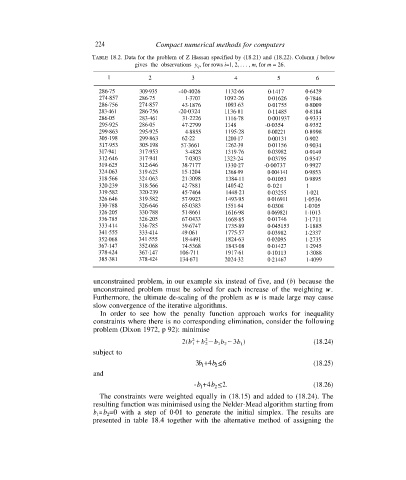
224 Compact numerical methods for computers
TABLE 18.2. Data for the problem of Z Hassan specified by (18.21) and (18.22). Column j below
gives the observations y ij , for rows i=1, 2, . . . , m, for m = 26.
1 2 3 4 5 6
286·75 309·935 -40·4026 1132·66 0·1417 0·6429
274·857 286·75 1·3707 1092·26 0·01626 0·7846
286·756 274·857 43·1876 1093·63 0·01755 0·8009
283·461 286·756 -20·0324 1136·81 0·11485 0·8184
286·05 283·461 31·2226 1116·78 0·001937 0·9333
295·925 286·05 47·2799 1148 -0·0354 0·9352
299·863 295·925 4·8855 1195·28 0·00221 0·8998
305·198 299·863 62·22 1200·17 0·00131 0·902
317·953 305·198 57·3661 1262·39 0·01156 0·9034
317·941 317·953 3·4828 1319·76 0·03982 0·9149
312·646 317·941 7·0303 1323·24 0·03795 0·9547
319·625 312·646 38·7177 1330·27 -0·00737 0·9927
324·063 319·625 15·1204 1368·99 0·004141 0·9853
318·566 324·063 21·3098 1384·11 0·01053 0·9895
320·239 318·566 42·7881 1405·42 0·021 1
319·582 320·239 45·7464 1448·21 0·03255 1·021
326·646 319·582 57·9923 1493·95 0·016911 1·0536
330·788 326·646 65·0383 1551·94 0·0308 1·0705
326·205 330·788 51·8661 1616·98 0·069821 1·1013
336·785 326·205 67·0433 1668·85 0·01746 1·1711
333·414 336·785 39·6747 1735·89 0·045153 1·1885
341·555 333·414 49·061 1775·57 0·03982 1·2337
352·068 341·555 18·4491 1824·63 0·02095 1·2735
367·147 352·068 74·5368 1843·08 0·01427 1·2945
378·424 367·147 106·711 1917·61 0·10113 1·3088
385·381 378·424 134·671 2024·32 0·21467 1·4099

unconstrained problem, in our example six instead of five, and (b) because the
unconstrained problem must be solved for each increase of the weighting w.
Furthermore, the ultimate de-scaling of the problem as w is made large may cause
slow convergence of the iterative algorithms.
In order to see how the penalty function approach works for inequality
constraints where there is no corresponding elimination, consider the following
problem (Dixon 1972, p 92): minimise

(18.24)
subject to
3b +4b <6 (18.25)
1
2
and
-b +4b <2. (18.26)
1
2
The constraints were weighted equally in (18.15) and added to (18.24). The
resulting function was minimised using the Nelder-Mead algorithm starting from
b = b =0 with a step of 0·01 to generate the initial simplex. The results are
2
1
presented in table 18.4 together with the alternative method of assigning the