Page 262 - Compact Numerical Methods For Computers

Conjugate gradients method in linear algebra 249
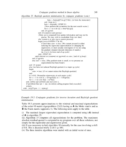
Algorithm 25. Rayleigh quotient minimisation by conjugate gradients (cont.)
beta := beta+g[i]*(w-g[i]*xbt); {to form the numerator}
end; {loop on i}
beta := beta/tabt; {STEP 23}
{Now perform the recurrence for the next search vector.}
for i := 1 to n do t[i] := beta*t[i]-g[i];
end; {if gg>tol}
end {if (count<n) and (pn<rq)}
{Note: pn is computed from update information and may not be
precise. We may wish to recalculate from raw data}
else {count=n or pn>=rq so cannot proceed}
begin {rest of STEPS 17 & 18}
if itn=l then conv := true; {We cannot proceed in either
reducing the eigenvalue approximation or changing the
eigenvector, so must assume convergence if we are using
the gradient (steepest descent) direction of search.}
itn := n+l; {to force end of cg cycle}
end; {STEP 24}
until (itn>=n) or (count=n) or (gg<=tol) or conv; {end of cg loop}
end {if gg>tol}
else conv := true; {The gradient norm is small, so we presume an
eigensolution has been found.}
end {if rq<pa}
else {we have not reduced Rayleigh quotient in a major cg cycle}
begin
conv := true; {if we cannot reduce the Rayleigh quotient}
end;
ta := 0.0; {Normalize eigenvector at each major cycle}
for i := 1 to n do ta := ta+sqr(X[i]); ta := 1.0/sqrt(ta);
for i := 1 to n do X[i] := ta*X[i];
end; {while (ipr<=itlimit) and (not conv) }
if ipr>itlimit then ipr := -ipr; {to inform calling program limit exceeded}
writeln;
end; {alg25.pas == rqmcg}

Example 19.3. Conjugate gradients for inverse iteration and Rayleigh quotient
minimisation
Table 19.3 presents approximations to the minimal and maximal eigensolutions
of the order-10 matrix eigenproblem (2.63) having as A the Moler matrix and as
B the Frank matrix (appendix 1). The following notes apply to the table.
(i) The maximal (largest eigenvalue) eigensolution is computed using (-A) instead
of A in algorithm 25.
(ii) Algorithm 15 computes all eigensolutions for the problem. The maximum
absolute residual quoted is computed in my program over all these solutions, not
simply for the eigenvalue and eigenvector given.
(iii) It was necessary to halt algorithm 10 manually for the case involving a shift
of 8·8. This is discussed briefly in §9.3 (p 109).
(iv) The three iterative algorithms were started with an initial vector of ones.