Page 50 - Complementarity and Variational Inequalities in Electronics

40 Complementarity and Variational Inequalities in Electronics

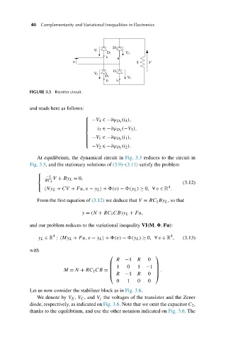
FIGURE 3.5 Rectifier circuit.

and reads here as follows:

⎧
(i 4 ),
⎪ −V 4 ∈−∂ϕ D 4
⎪
⎪
⎪
⎨ (−V 3 ),
i 3 ∈−∂ϕ D 3
(i 1 ),
⎪
⎪ −V 1 ∈−∂ϕ D 1
⎪
⎪
(i 2 ).
⎩
−V 2 ∈−∂ϕ D 2
At equilibrium, the dynamical circuit in Fig. 3.3 reduces to the circuit in
Fig. 3.5, and the stationary solutions of (3.9)–(3.11) satisfy the problem
⎧
−1
⎨ V + By L = 0,
RC 1
(3.12)
Ny L + CV + Fu,v − y L + (v) − (y L ) ≥ 0, ∀ v ∈ R .
⎩ 4
From the first equation of (3.12) we deduce that V = RC 1 By L , so that
y = (N + RC 1 CB)y L + Fu,
and our problem reduces to the variational inequality VI(M, ,Fu):
4
4
y L ∈ R : My L + Fu,v − y L + (v) − (y L ) ≥ 0, ∀ v ∈ R , (3.13)
with
⎛ ⎞
R −1 R 0
⎜ 1 0 1 ⎟
⎜
⎟.
−1 ⎟
⎝ R −1 R 0 ⎠
M = N + RC 1 CB = ⎜
0 1 0 0
Let us now consider the stabilizer block as in Fig. 3.6.
We denote by V E , V C , and V z the voltages of the transistor and the Zener
diode, respectively, as indicated on Fig. 3.6. Note that we omit the capacitor C 2 ,
thanks to the equilibrium, and use the other notation indicated on Fig. 3.6.The