
Page 107 - Computational Colour Science Using MATLAB
P. 107
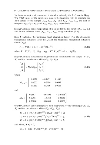
94 CHROMATIC-ADAPTATION TRANSFORMS AND COLOUR APPEARANCE
361 column matrix of normalized tristimulus values by the 363 matrix M BFD .
The XYZ values of the sample are used with Equations (6.6) to compute the
RGB values for the sample; X WT , Y WT , Z WT and X WR , Y WR , Z WR are used to
compute R WT , G WT , B WT and R WR , G WR , B WR , respectively.
Step 2: Calculate the corresponding RGB values for the test sample (R , G , B )
C
C
C
and for the reference white (R WC , G WC , B WC ) using Equations (6.10).
Step 3: Calculate the luminance level adaptation factor (F ), the chromatic
L
background induction factor (N ) and the brightness background induction
CB
factor (N ),
BB
4 4 2 1=3
F L ¼ K ðL A Þþ 0:1ð1 K Þ ð5L A Þ , ð6:16Þ
where K ¼ 1/(5L +1), N ¼ N ¼ 0.725(1/n) 0.2 and n ¼ Y /Y .
A CB BB B W
Step 4: Calculate the corresponding tristimulus values for the test sample (R , G ,
0
0
B ) and for the reference white (R , G , B ),
0
0
0
0
W
W
W
2 3 2 3
R 0 R C Y
G 5 ¼ M H M G C Y 5,
6 0 7 1 6 7
4 BFD 4 ð6:17Þ
B 0 B C Y
where
2 3
0:9870 0:1471 0:1600
M 1 6 0:4323 0:5184 7
BFD ¼ 4 0:0493 5
0:0085 0:0400 0:9685
and
0:38971 0:68898 0:07868
2 3
0:22981 1:18340 0:04641 5.
6 7
M H ¼ 4
0:00000 0:00000 1:00000
Step 5: Calculate the cone responses after adaptation for the test sample (R , G ,
0
0
a
a
B ) and for the reference white (R aW , G 0 aW , B aW ),
0
0
0
a
0:73 0:73
0 0 0 þ 2,
R a ¼ 1 þ½40ðF L R =100Þ =½ðF L R =100Þ
0:73 0:73
0 0 0 þ 2,
G a ¼ 1 þ½40ðF L G =100Þ =½F L G =100Þ ð6:18Þ
0:73 0:73
0 0 0 þ 2,
B a ¼ 1 þ½40ðF L B =100Þ =½ðF L B =100Þ
and where, if R 5 0,
0
a
0:73 0:73
0 0 0 þ 2.
R a ¼ 1 ½40ð R =100Þ =½ð R =100Þ