Page 108 - Computational Colour Science Using MATLAB

CAMS 95

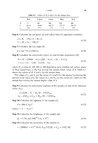
Table 6.1 Values of H, h and e for the unique hues
Red Yellow Green Blue Red

H 0 100 200 300 400
h 20.14 90.00 164.25 237.53 380.14
e 0.8 0.7 1.0 1.2 0.8

Step 6: Calculate the red-green (a) and yellow-blue (b) opponent correlates,

a ¼ R a 12G a =11 þ B a =11,
0
0
0
b ¼ðR a þ G a 2B a Þ=9. ð6:19Þ
0
0
0
Step 7: Calculate the hue angle (h),
1
h ¼ tan ðb=aÞð180=pÞ. ð6:20Þ
Step 8: Calculate the eccentricity factor (e) and the hue quadrature (H),
H ¼ H 1 þ½100ðh h 1 Þ=e 1 Š=½ðh h 1 Þ=e 1 þðh 2 h 1 Þ=e 2 Š,
e ¼ e 1 þðe 2 e 1 Þðh h 1 Þ=ðh 2 h 1 Þ, ð6:21Þ

where H is either 0, 100, 200 or 300 depending upon whether red, yellow, green
1
or blue respectively, is the hue having the nearest lower value of h. Table 6.1
shows the values of H, h and e for the unique hues.
The values of e and h are the values of e and h for the unique hue having the
1
1
nearest lower value of h; the values of e and h are the values of e and h for the
2
2
unique hue having the nearest higher value of h.
Step 9: Calculate the achromatic response of the sample (A) and of the reference
white (A ),
W
A ¼½2R þ G þ B =20 2:05ŠN BB,
0
0
0
a a a
ð6:22Þ
A W ¼½2R 0 þ G 0 þ B 0 =20 2:05ŠN BB .
aW aW aW
Step 10: Calculate the lightness of the sample (J),
cz
J ¼ 100ðA=A W Þ , ð6:23Þ
1/2
where z ¼ 1+ F n .
LL
Step 11: Calculate the brightness of the sample (Q),
0:67 0:9
Q ¼ð1:24=cÞðJ=100Þ ðA W þ 3Þ . ð6:24Þ
Step 12: Calculate the saturation of the sample (s),
2 2 1=2 10eN C N BB =13Š=½R þ G 0 þ 21B =20Š.
0
0
s ¼½5000ða þ b Þ a aW a ð6:25Þ